|
Peano
|
|
Peano
|
Namespaces | |
| namespace | bottomFriction |
| namespace | coriolisForce |
| namespace | FrictionLaws |
| namespace | GulfOfMexico |
| namespace | meteotsunami |
| namespace | R1 |
Enumerations | |
| enum | RiemannStructure { DrySingleRarefaction , SingleRarefactionDry , ShockShock , ShockRarefaction , RarefactionShock , RarefactionRarefaction } |
| The Riemann-struture of the homogeneous Riemann-problem. More... | |
| enum class | WetDryState { DryDry , WetWet , WetDryInundation , WetDryWall , WetDryWallInundation , DryWetInundation , DryWetWall , DryWetWallInundation } |
Functions | |
| template<class T > | |
| static GPU_CALLABLE_METHOD RiemannStructure | determineRiemannStructure (const T &hLeft, const T &hRight, const T &uLeft, const T &uRight) |
| template<class T > | |
| static GPU_CALLABLE_METHOD void | solveLinearEquation (const T matrix[3][3], const T b[3], T x[3]) |
| template<class T > | |
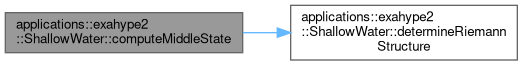
| static GPU_CALLABLE_METHOD T | computeMiddleState (const T &hLeft, const T &hRight, const T &uLeft, const T &uRight, RiemannStructure &riemannStructure, T *middleSpeeds) |
| template<class T > | |
| static GPU_CALLABLE_METHOD WetDryState | determineWetDryState (T &hLeft, T &huLeft, T &hvLeft, T &uLeft, T &vLeft, T &bLeft, T &hRight, T &huRight, T &hvRight, T &uRight, T &vRight, T &bRight, T &hMiddle, WetDryState &wetDryState, RiemannStructure &riemannStructure, T *middleSpeeds) |
| template<class T > | |
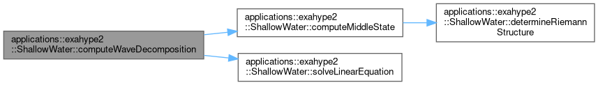
| static GPU_CALLABLE_METHOD void | computeWaveDecomposition (T &hLeft, T &huLeft, T &uLeft, T &vLeft, T &bLeft, T &hRight, T &huRight, T &uRight, T &vRight, T &bRight, T &hMiddle, const T &sqrtGhLeft, const T &sqrtGhRight, const T &sqrthLeft, const T &sqrthRight, const T &sqrtG, WetDryState &wetDryState, RiemannStructure &riemannStructure, T fWaves[3][3], T waveSpeeds[3], T *middleSpeeds) |
| template<class T , class Shortcuts > | |
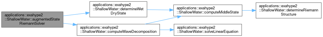
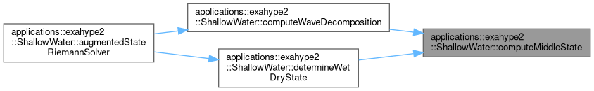
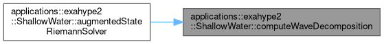
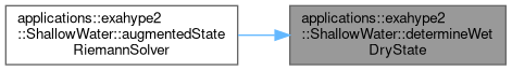
| static GPU_CALLABLE_METHOD double | augmentedStateRiemannSolver (const T *const NOALIAS QL, const T *const NOALIAS QR, const tarch::la::Vector< DIMENSIONS, double > &x, const tarch::la::Vector< DIMENSIONS, double > &h, const double t, const double dt, const int normal, T *const NOALIAS FL, T *const NOALIAS FR) |
| A implementation of the augmented state Riemann solver from David L. | |
| template<class T , class Shortcuts > | |
| static GPU_CALLABLE_METHOD double | fWaveRiemannSolver (const T *const NOALIAS QL, const T *const NOALIAS QR, const tarch::la::Vector< DIMENSIONS, double > &x, const tarch::la::Vector< DIMENSIONS, double > &h, const double t, const double dt, const int normal, T *const NOALIAS FL, T *const NOALIAS FR) |
| F-Wave Riemann Solver for the Shallow Water Equation. | |
| template<class T > | |
| static GPU_CALLABLE_METHOD double | middleHeightEstimation (const T &hLeft, const T &hRight, const T &uLeft, const T &uRight) |
| template<class T , class Shortcuts > | |
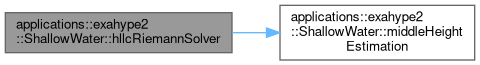
| static GPU_CALLABLE_METHOD double | hllcRiemannSolver (const T *const NOALIAS QL, const T *const NOALIAS QR, const tarch::la::Vector< DIMENSIONS, double > &x, const tarch::la::Vector< DIMENSIONS, double > &h, const double t, const double dt, const int normal, T *const NOALIAS FL, T *const NOALIAS FR) |
| Implementation of a HLLC solver utilising Einfeldt speeds for the outer wave speed estimates. | |
| template<class T , class Shortcuts > | |
| static GPU_CALLABLE_METHOD double | hllemRiemannSolver (const T *const NOALIAS QL, const T *const NOALIAS QR, const tarch::la::Vector< DIMENSIONS, double > &x, const tarch::la::Vector< DIMENSIONS, double > &h, const double t, const double dt, const int normal, T *const NOALIAS FL, T *const NOALIAS FR) |
| A new formulation of the HLLEM Riemann solver for the Shallow Water Equation with support for inundation. | |
| template<class T , class Shortcuts > | |
| static GPU_CALLABLE_METHOD double | llfRiemannSolver (const T *const NOALIAS QL, const T *const NOALIAS QR, const tarch::la::Vector< DIMENSIONS, double > &x, const tarch::la::Vector< DIMENSIONS, double > &h, const double t, const double dt, const int normal, T *const NOALIAS FL, T *const NOALIAS FR) |
| Implementation of a LLF-Riemann Solver with Hydrostatic Reconstruction for. | |
| template<class T , class Shortcuts , int NumberOfUnknowns> | |
| static GPU_CALLABLE_METHOD void | flux (const T *const NOALIAS Q, const tarch::la::Vector< DIMENSIONS, double > &x, const tarch::la::Vector< DIMENSIONS, double > &h, const double t, const double dt, const int normal, T *const NOALIAS F) |
| template<class T , class Shortcuts > | |
| static GPU_CALLABLE_METHOD double | maxEigenvalue (const T *const NOALIAS Q, const tarch::la::Vector< DIMENSIONS, double > &x, const tarch::la::Vector< DIMENSIONS, double > &h, const double t, const double dt, const int normal) |
| template<class T , class Shortcuts , int NumberOfUnknowns> | |
| static GPU_CALLABLE_METHOD void | nonconservativeProduct (const T *const NOALIAS Q, const T *const NOALIAS deltaQ, const tarch::la::Vector< DIMENSIONS, double > &x, const tarch::la::Vector< DIMENSIONS, double > &h, const double t, const double dt, const int normal, T *const NOALIAS BTimesDeltaQ) |
| template<class T , class Shortcuts , class Quadrature , int NumberOfUnknowns, int NumberOfAuxiliaryVariables, int Order> | |
| static GPU_CALLABLE_METHOD void | rusanovRiemannSolverADERDG (const T *const NOALIAS QL, const T *const NOALIAS QR, const tarch::la::Vector< DIMENSIONS, double > &x, const tarch::la::Vector< DIMENSIONS, double > &h, const double t, const double dt, const int normal, T *const NOALIAS FL, T *const NOALIAS FR) |
| template<class T , class Shortcuts , int NumberOfUnknowns, int NumberOfAuxiliaryVariables> | |
| static GPU_CALLABLE_METHOD double | rusanovRiemannSolverFV (const T *const NOALIAS QL, const T *const NOALIAS QR, const tarch::la::Vector< DIMENSIONS, double > &x, const tarch::la::Vector< DIMENSIONS, double > &h, const double t, const double dt, const int normal, T *const NOALIAS FL, T *const NOALIAS FR) |
Variables | |
| constexpr double | g = landslide::g |
| constexpr double | hThreshold = landslide::hThreshold |
| constexpr int | NEWTON_ITER = 1 |
| constexpr double | NEWTON_TOL = 1e-5 |
| constexpr double | CONVERGENCE_TOL = 1e-5 |
| constexpr double | ZERO_TOL = 1e-5 |
The Riemann-struture of the homogeneous Riemann-problem.
| Enumerator | |
|---|---|
| DrySingleRarefaction | |
| SingleRarefactionDry | |
| ShockShock | |
| ShockRarefaction | |
| RarefactionShock | |
| RarefactionRarefaction | |
Definition at line 11 of file AugmentedStateRiemannSolver.cpph.
|
strong |
| Enumerator | |
|---|---|
| DryDry | |
| WetWet | |
| WetDryInundation | |
| WetDryWall | |
| WetDryWallInundation | |
| DryWetInundation | |
| DryWetWall | |
| DryWetWallInundation | |
Definition at line 6 of file WetDryState.h.
|
static |
A implementation of the augmented state Riemann solver from David L.
George modified for 2D scenarios and for compatibility for the ExaHyPE 2 project
Main scientific source for the implementation: @article{George2008, title = {Augmented Riemann solvers for the shallow water equations over variable topography with steady states and inundation}, journal = {Journal of Computational Physics}, volume = {227}, number = {6}, pages = {3089-3113}, year = {2008}, issn = {0021-9991}, doi = {https://doi.org/10.1016/j.jcp.2007.10.027}, url = {https://www.sciencedirect.com/science/article/pii/S0021999107004767}, author = {David L. George}, keywords = {Shallow water equations, Hyperbolic conservation laws, Finite volume methods, Godunov methods, Riemann solvers, Wave propagation, Shock capturing methods, Tsunami modeling}, abstract = {We present a class of augmented approximate Riemann solvers for the shallow water equations in the presence of a variable bottom surface. These belong to the class of simple approximate solvers that use a set of propagating jump discontinuities, or waves, to approximate the true Riemann solution. Typically, a simple solver for a system of m conservation laws uses m such discontinuities. We present a four wave solver for use with the the shallow water equations—a system of two equations in one dimension. The solver is based on a decomposition of an augmented solution vector—the depth, momentum as well as momentum flux and bottom surface. By decomposing these four variables into four waves the solver is endowed with several desirable properties simultaneously. This solver is well-balanced: it maintains a large class of steady states by the use of a properly defined steady state wave—a stationary jump discontinuity in the Riemann solution that acts as a source term. The form of this wave is introduced and described in detail. The solver also maintains depth non-negativity and extends naturally to Riemann problems with an initial dry state. These are important properties for applications with steady states and inundation, such as tsunami and flood modeling. Implementing the solver with LeVeque’s wave propagation algorithm [R.J. LeVeque, Wave propagation algorithms for multi-dimensional hyperbolic systems, J. Comput. Phys. 131 (1997) 327–335] is also described. Several numerical simulations are shown, including a test problem for tsunami modeling.} }
Additional information about the solver can be found here: @book{George2006, title={Finite volume methods and adaptive refinement for tsunami propagation and inundation}, author={George, David L}, year={2006}, publisher={University of Washington} }
Additionally, this solver has been based on two reference implementations: The Clawpack implementation written in Fortran, which incorporates additional modifications for stability and 2D domains (especially the subroutine riemann_aug_JCP): https://github.com/clawpack/riemann/blob/master/src/rpn2_sw_aug.f90
And another C++ implementation, where the structure of the code is based on in some parts: https://github.com/TUM-I5/SWE-Solvers/blob/master/Source/AugRieSolver.hpp
Further sources utilized by https://github.com/TUM-I5/swe-Solvers/blob/master/Source/AugRieSolver.hpp:
@book{LeVeque2002, title={Finite volume methods for hyperbolic problems}, author={LeVeque, Randall J}, volume={31}, year={2002}, publisher={Cambridge university press} }
@webpage{LeVeque2011, Author = {LeVeque, R. J.}, Lastchecked = {January, 05, 2011}, Title = {Clawpack Sofware}, Url = {https://github.com/clawpack/clawpack-4.x/blob/master/geoclaw/2d/lib} }
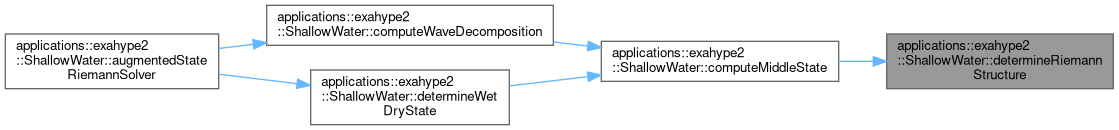
Definition at line 794 of file AugmentedStateRiemannSolver.cpph.
References computeWaveDecomposition(), and determineWetDryState().
|
static |
Definition at line 82 of file AugmentedStateRiemannSolver.cpph.
References determineRiemannStructure(), g, hThreshold, NEWTON_ITER, NEWTON_TOL, RarefactionRarefaction, RarefactionShock, ShockRarefaction, and ShockShock.
Referenced by computeWaveDecomposition(), and determineWetDryState().
|
static |
Definition at line 344 of file AugmentedStateRiemannSolver.cpph.
References computeMiddleState(), CONVERGENCE_TOL, DryWetWall, g, hThreshold, NEWTON_ITER, RarefactionRarefaction, RarefactionShock, ShockRarefaction, solveLinearEquation(), WetDryWall, and ZERO_TOL.
Referenced by augmentedStateRiemannSolver().
|
static |
Definition at line 22 of file AugmentedStateRiemannSolver.cpph.
References DrySingleRarefaction, g, hThreshold, RarefactionRarefaction, RarefactionShock, ShockRarefaction, ShockShock, and SingleRarefactionDry.
Referenced by computeMiddleState().
|
static |
Definition at line 247 of file AugmentedStateRiemannSolver.cpph.
References computeMiddleState(), DryDry, DryWetInundation, DryWetWall, DryWetWallInundation, hThreshold, WetDryInundation, WetDryWall, WetDryWallInundation, and WetWet.
Referenced by augmentedStateRiemannSolver().

|
static |
|
static |
F-Wave Riemann Solver for the Shallow Water Equation.
Note: This solver does not support inundation. For dry cells, we assume an infinitely high solid wall at the shore-line, which is equivalent to reflecting boundary conditions. Thus no water is able to pass the shoreline, and we have to assure that the particle velocity at the boundary is zero.
Literature:
@article{Bale2002, title={A wave propagation method for conservation laws and balance laws with spatially varying flux functions}, author={Bale, D.S. and LeVeque, R.J. and Mitran, S. and Rossmanith, J.A.}, journal={SIAM Journal on Scientific Computing}, volume={24}, number={3}, pages={955–978}, year={2002}, publisher={Citeseer}}
@book{LeVeque2002, Author = {LeVeque, R. J.}, Date-Added = {2011-09-13 14:09:31 +0000}, Date-Modified = {2011-10-31 09:46:40 +0000}, Publisher = {Cambridge University Press}, Title = {Finite Volume Methods for Hyperbolic Problems}, Volume = {31}, Year = {2002}}
@webpage{LeVeque2011, Author = {LeVeque, R. J.}, Lastchecked = {January, 05, 2011}, Title = {Clawpack Sofware}, Url = {https://github.com/clawpack/clawpack-4.x/blob/master/geoclaw/2d/lib}}
Wet/dry state of our Riemann-problem
Wave speeds of the f-waves
Definition at line 5 of file FWaveRiemannSolver.cpph.
References ZERO_TOL.
|
static |
Implementation of a HLLC solver utilising Einfeldt speeds for the outer wave speed estimates.
In order to account for varying bathymetry and steady states, the solver also utilises a local hydrostatic reconstruction approach.
The basic HLLC approach and the middle height based wave speed estimation process is described in the following scientific sources:
@article{Toro2019, title = {The {HLLC} {Riemann} solver}, volume = {29}, issn = {1432-2153}, url = {https://doi.org/10.1007/s00193-019-00912-4}, doi = {10.1007/s00193-019-00912-4}, abstract = {The HLLC (Harten–Lax–van Leer contact) approximate Riemann solver for computing solutions to hyperbolic systems by means of finite volume and discontinuous Galerkin methods is reviewed. HLLC was designed, as early as 1992, as an improvement to the classical HLL (Harten–Lax–van Leer) Riemann solver of Harten, Lax, and van Leer to solve systems with three or more characteristic fields, in order to avoid the excessive numerical dissipation of HLL for intermediate characteristic fields. Such numerical dissipation is particularly evident for slowly moving intermediate linear waves and for long evolution times. High-order accurate numerical methods can, to some extent, compensate for this shortcoming of HLL, but it is a costly remedy and for stationary or nearly stationary intermediate waves such compensation is very difficult to achieve in practice. It is therefore best to resolve the problem radically, at the first-order level, by choosing an appropriate numerical flux. The present paper is a review of the HLLC scheme, starting from some historical notes, going on to a description of the algorithm as applied to some typical hyperbolic systems, and ending with an overview of some of the most significant developments and applications in the last 25 years.}, number = {8}, journal = {Shock Waves}, author = {Toro, E. F.}, month = nov, year = {2019}, pages = {1065–1082}, }
In the following book, especially section 11.4 HLLC Riemann Solvers describes the basic HLLC solver:
@book{Toro2024, title={Computational Algorithms for Shallow Water Equations}, author={Toro, Eleuterio F}, year={2024}, publisher={Springer Cham} }
@article{Fraccarollo1995, author = {Luigi Fraccarollo and Eleuterio F. Toro}, title = {Experimental and numerical assessment of the shallow water model for two-dimensional dam-break type problems}, journal = {Journal of Hydraulic Research}, volume = {33}, number = {6}, pages = {843–864}, year = {1995}, publisher = {IAHR Website}, doi = {10.1080/00221689509498555}, URL = { https://doi.org/10.1080/00221689509498555 }, eprint = { https://doi.org/10.1080/00221689509498555 } }
The local hydrostatic reconstruction approach, used for:
@article{Clain2016, author = {Clain, S. and Reis, C. and Costa, R. and Figueiredo, J. and Baptista, M. A. and Miranda, J. M.}, title = {Second-order finite volume with hydrostatic reconstruction for tsunami simulation}, journal = {Journal of Advances in Modeling Earth Systems}, volume = {8}, number = {4}, pages = {1691-1713}, keywords = {second-order, finite volume scheme, hydrostatic reconstruction, nonconservative flux, application to tsunami}, doi = {https://doi.org/10.1002/2015MS000603}, url = {https://agupubs.onlinelibrary.wiley.com/doi/abs/10.1002/2015MS000603}, eprint = {https://agupubs.onlinelibrary.wiley.com/doi/pdf/10.1002/2015MS000603}, abstract = {Abstract Tsunami modeling commonly accepts the shallow water system as governing equations where the major difficulty is the correct treatment of the nonconservative term due to bathymetry variations. The finite volume method for solving the shallow water equations with such source terms has received great attention in the two last decades. The built-in conservation property, the capacity to correctly treat discontinuities, and the ability to handle complex bathymetry configurations preserving some steady state configurations (well-balanced scheme) make the method very efficient. Nevertheless, it is still a challenge to build an efficient numerical scheme, with very few numerical artifacts (e.g., small numerical diffusion, correct propagation of the discontinuities, accuracy, and robustness), to be used in an operational environment, and that is able to better capture the dynamics of the wet-dry interface and the physical phenomena that occur in the inundation area. In the first part of this paper, we present a new second-order finite volume code. The code is developed for the shallow water equations with a nonconservative term based on the hydrostatic reconstruction technology to achieve a well-balanced scheme and an adequate dry/wet interface treatment. A detailed presentation of the numerical method is given. In the second part of the paper, we highlight the advantages of the new numerical technique. We benchmark the numerical code against analytical, experimental, and field results to assess the robustness and the accuracy of the numerical code. Finally, we use the 28 February 1969 North East Atlantic tsunami to check the performance of the code with real data.}, year = {2016} }
@article{Audusse2004, author = {Audusse, Emmanuel and Bouchut, Fran{c}ois and Bristeau, Marie-Odile and Klein, Rupert and Perthame, Beno\i{}⁁t}, title = {A Fast and Stable Well-Balanced Scheme with Hydrostatic Reconstruction for Shallow Water Flows}, journal = {SIAM Journal on Scientific Computing}, volume = {25}, number = {6}, pages = {2050-2065}, year = {2004}, doi = {10.1137/S1064827503431090}, URL = { https://doi.org/10.1137/S1064827503431090 }, eprint = { https://doi.org/10.1137/S1064827503431090 } , abstract = { We consider the Saint-Venant system for shallow water flows, with nonflat bottom. It is a hyperbolic system of conservation laws that approximately describes various geophysical flows, such as rivers, coastal areas, and oceans when completed with a Coriolis term, or granular flows when completed with friction. Numerical approximate solutions to this system may be generated using conservative finite volume methods, which are known to properly handle shocks and contact discontinuities. However, in general these schemes are known to be quite inaccurate for near steady states, as the structure of their numerical truncation errors is generally not compatible with exact physical steady state conditions. This difficulty can be overcome by using the so-called well-balanced schemes. We describe a general strategy, based on a local hydrostatic reconstruction, that allows us to derive a well-balanced scheme from any given numerical flux for the homogeneous problem. Whenever the initial solver satisfies some classical stability properties, it yields a simple and fast well-balanced scheme that preserves the nonnegativity of the water height and satisfies a semidiscrete entropy inequality. } }
@Inbook{Ortleb2022, author="Ortleb, Sigrunand Lambrechts, Jonathan and K{\"a}rn{\"a}, Tuomas", editor="Schuttelaars, Henk and Heemink, Arnold and Deleersnijder, Eric", title="Wetting and drying Procedures for Shallow Water Simulations", bookTitle="The Mathematics of Marine Modelling: Water, Solute and Particle Dynamics in Estuaries and Shallow Seas", year="2022", publisher="Springer International Publishing", address="Cham", pages="287--314", abstract="In the coastal zone, the alternating exposure and submerging of the seabed is an important feature in coastal engineering and marine ecosystems. The wetting and drying of shallow regions challenges the numerical simulation in terms of robustness, efficiency, and the preservation of physical properties. Considering a physically sound representation, desired numerical properties include positivity preservation with respect to the water depth, local and global mass conservation, well-balancedness with respect to lake at rest steady states, and avoidance of artificial pressure gradients. This chapter focuses on recent numerical methods on fixed computational grids based on the depth-averaged shallow water equations where we review and discuss the classes of finite volume methods and discontinuous Galerkin schemes and their respective wetting and drying treatment. In addition, the numerical approaches are classified with respect to either explicit or implicit time integration, and we discuss the advantages and disadvantages accompanying these two alternatives.", isbn="978-3-031-09559-7", doi="10.1007/978-3-031-09559-7_11", url="https://doi.org/10.1007/978-3-031-09559-7_11" }
The Kurganov desingularization is described in: @article{Kurganov2007, title={A second-order well-balanced positivity preserving central-upwind scheme for the Saint-Venant system}, author={Kurganov, Alexander and Petrova, Guergana}, year={2007} }
Some details about more sophisticated middle height estimations processes can be found in: @article{George2008, title = {Augmented Riemann solvers for the shallow water equations over variable topography with steady states and inundation}, journal = {Journal of Computational Physics}, volume = {227}, number = {6}, pages = {3089-3113}, year = {2008}, issn = {0021-9991}, doi = {https://doi.org/10.1016/j.jcp.2007.10.027}, url = {https://www.sciencedirect.com/science/article/pii/S0021999107004767}, author = {David L. George}, keywords = {Shallow water equations, Hyperbolic conservation laws, Finite volume methods, Godunov methods, Riemann solvers, Wave propagation, Shock capturing methods, Tsunami modeling}, abstract = {We present a class of augmented approximate Riemann solvers for the shallow water equations in the presence of a variable bottom surface. These belong to the class of simple approximate solvers that use a set of propagating jump discontinuities, or waves, to approximate the true Riemann solution. Typically, a simple solver for a system of m conservation laws uses m such discontinuities. We present a four wave solver for use with the the shallow water equations—a system of two equations in one dimension. The solver is based on a decomposition of an augmented solution vector—the depth, momentum as well as momentum flux and bottom surface. By decomposing these four variables into four waves the solver is endowed with several desirable properties simultaneously. This solver is well-balanced: it maintains a large class of steady states by the use of a properly defined steady state wave—a stationary jump discontinuity in the Riemann solution that acts as a source term. The form of this wave is introduced and described in detail. The solver also maintains depth non-negativity and extends naturally to Riemann problems with an initial dry state. These are important properties for applications with steady states and inundation, such as tsunami and flood modeling. Implementing the solver with LeVeque’s wave propagation algorithm [R.J. LeVeque, Wave propagation algorithms for multi-dimensional hyperbolic systems, J. Comput. Phys. 131 (1997) 327–335] is also described. Several numerical simulations are shown, including a test problem for tsunami modeling.} } and: https://github.com/clawpack/riemann/blob/master/src/rpn2_sw_aug.f90
Definition at line 71 of file HLLCRiemannSolver.cpph.
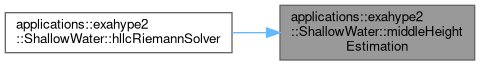
References middleHeightEstimation().
|
static |
A new formulation of the HLLEM Riemann solver for the Shallow Water Equation with support for inundation.
Literature:
@article{Dumbser2016, title = {A new efficient formulation of the HLLEM Riemann solver for general conservative and non-conservative hyperbolic systems}, journal = {Journal of Computational Physics}, volume = {304}, pages = {275-319}, year = {2016}, issn = {0021-9991}, doi = {https://doi.org/10.1016/j.jcp.2015.10.014}, url = {https://www.sciencedirect.com/science/article/pii/S0021999115006786}, author = {Michael Dumbser and Dinshaw S. Balsara}}
@article{Kurganov2007, title = {A Second-Order Well-Balanced Positivity Preserving Central-Upwind Scheme for the Saint-Venant System}, year = {2007}, month = {03}, pages = {}, volume = {5}, journal = {Communications in mathematical sciences}, author = {Kurganov, Alexander and Petrova, G.}, doi = {10.4310/CMS.2007.v5.n1.a6}}
Definition at line 5 of file HLLEMRiemannSolver.cpph.
|
static |
Implementation of a LLF-Riemann Solver with Hydrostatic Reconstruction for.
Based on the following papers:
Definition at line 5 of file LLFRiemannSolver.cpph.
|
static |
|
static |
Definition at line 10 of file HLLCRiemannSolver.cpph.
References g, hThreshold, NEWTON_ITER, and NEWTON_TOL.
Referenced by hllcRiemannSolver().
|
static |
|
static |
Definition at line 5 of file RusanovRiemannSolver.cpph.
|
static |
|
static |
Definition at line 58 of file AugmentedStateRiemannSolver.cpph.
Referenced by computeWaveDecomposition().

|
constexpr |
Definition at line 7 of file AugmentedStateRiemannSolver.cpph.
Referenced by computeWaveDecomposition().
|
constexpr |
Definition at line 55 of file PDE.h.
Referenced by computeMiddleState(), computeWaveDecomposition(), determineRiemannStructure(), and middleHeightEstimation().
|
constexpr |
Definition at line 56 of file PDE.h.
Referenced by computeMiddleState(), computeWaveDecomposition(), determineRiemannStructure(), determineWetDryState(), and middleHeightEstimation().
|
constexpr |
Definition at line 5 of file AugmentedStateRiemannSolver.cpph.
Referenced by computeMiddleState(), computeWaveDecomposition(), and middleHeightEstimation().
|
constexpr |
Definition at line 6 of file AugmentedStateRiemannSolver.cpph.
Referenced by computeMiddleState(), and middleHeightEstimation().
|
constexpr |
Definition at line 8 of file AugmentedStateRiemannSolver.cpph.
Referenced by computeWaveDecomposition(), and fWaveRiemannSolver().