Our First Implementation File

The astute reader might have noticed that before we built our project, there was one other file already present within the same directory: PlanarAcousticSolver.cpp.

We will be taking a look at this file next since, as you most likely have already guessed, it contains the implementation of our PDE.

Before we do this however, we will quickly define the PDE that is to come. As the name of the file will have already indicated, this is the two-dimensional acoustic equation which appears as follows:

\( \begin{equation*} \label{Acoustic_equation} \frac{\partial}{\partial t}\left( \begin{array}{lr} p \\ v_1 \\ v_2 \end{array} \right) + \nabla \begin{pmatrix} K_0 v_1 & K_0 v_2 \\ \frac{p}{\rho} & 0 \\ 0 & \frac{p}{\rho} \end{pmatrix} = \vec{0} \end{equation*} \)

where p is the pressure, and v_1 and v_2 are the velocity respectively in the x- and y-direction. It additionally uses two parameters which, for simplicity's sake we have assumed to remain constant over the domain. These are the density &rho=1 and the bulk modulus K0=4, which you can think of as the squishiness of the material (don't ask, we don't have time). In order to implement this equation, we need two things: a flux, and a maximal eigenvalue. The maximal eigenvalue is the greatest eigenvalue of the flux tensor, which is:

\( \begin{equation*} \label{Acoustic_eigenvalue} \lambda = \sqrt{\frac{K_0}{\rho}} \end{equation*} \)

This is required for the Riemann-solver (again, don't ask) and the time-stepping, and is implemented in the first function of our file:

double exahype2::training::acoustic::PlanarAcousticSolver::maxEigenvalue(
  [[maybe_unused]] const double* const NOALIAS   Q, // Q[3+0]
  [[maybe_unused]] const tarch::la::Vector<DIMENSIONS, double>& x,
  [[maybe_unused]] const tarch::la::Vector<DIMENSIONS, double>& h,
  [[maybe_unused]] const double                                 t,
  [[maybe_unused]] const double                                 dt,
  [[maybe_unused]] const int                                    normal
) {
  constexpr double K0  = 4.0;
  constexpr double rho = 1.0;
  const double c       = std::sqrt(4.0 / rho);
  return c;
}

Next is the flux, we have already defined it above, so let's look at the implementation:

void exahype2::training::acoustic::PlanarAcousticSolver::flux(
  [[maybe_unused]] const double* const NOALIAS   Q, // Q[3+0]
  [[maybe_unused]] const tarch::la::Vector<DIMENSIONS, double>& x,
  [[maybe_unused]] const tarch::la::Vector<DIMENSIONS, double>& h,
  [[maybe_unused]] const double                                 t,
  [[maybe_unused]] const double                                 dt,
  [[maybe_unused]] const int                                    normal,
  [[maybe_unused]] double* const NOALIAS F // F[3]
) {
  constexpr double K0  = 4.0;
  constexpr double rho = 1.0;

  switch (normal) {
  case 0: // Flux in x-direction
    F[Shortcuts::p]     = K0 * Q[Shortcuts::v + normal];
    F[Shortcuts::v + 0] = Q[Shortcuts::p] / rho;
    F[Shortcuts::v + 1] = 0.0;
    break;
  case 1: // Flux in y-direction
    F[Shortcuts::p]     = K0 * Q[Shortcuts::v + normal];
    F[Shortcuts::v + 0] = 0.0;
    F[Shortcuts::v + 1] = Q[Shortcuts::p] / rho;
  }
}

The flux has one component for each direction, which one we need is determined by the normal-parameter, and it depends on the values of the equation, which are found in Q. These two are sufficient to define the entire equation, a measly two functions and less than twenty lines of code. But we still need to define our initial conditions, we do so in the function appropriately-named initialCondition, and we prescribe a sinus for the initial conditions:

void exahype2::training::acoustic::PlanarAcousticSolver::initialCondition(
  [[maybe_unused]] double* const NOALIAS Q, // Q[3+0]
  [[maybe_unused]] const tarch::la::Vector<DIMENSIONS, double>& x,
  [[maybe_unused]] const tarch::la::Vector<DIMENSIONS, double>& h,
  [[maybe_unused]] const bool                                   gridIsConstructed
) {
  const double val = cos(-std::numbers::pi * (x[0] + x[1])); // Simple translation in positive diagonal direction

  Q[Shortcuts::v + 0] = val;
  Q[Shortcuts::v + 1] = val;

  constexpr double K0  = 4.0;
  constexpr double rho = 1.0;

  const double kr = std::sqrt(2 * K0 * rho); // These are defined by the eigenvector of the plane wave operator
  Q[Shortcuts::p]         = kr * val;
}

Finally, we would normally need to define boundary conditions to make our problem well-defined, but as we have specified periodic boundary conditions, this is not necessary here.

So, now that we've gone through all of this, let's go take a look at our results. These should be within the folder solutions and are stored in a custom format named peano-patch-file, which is essentially plain-text but allows for efficient parallel writing. In order to visualize this, we will first need to convert these files using following command:

python $PEANO_ROOT/python/peano4/visualisation/render.py solutions/solution-PlanarAcousticSolver.peano-patch-file

This converts the patch files to .vtu files, which we can read and visualise using e.g., ParaView:

paraview solutions/solution-PlanarAcousticSolver.pvd

If you've followed all of the steps until now, you should have following initial conditions for the pressure:

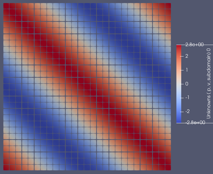
Can you tell us what these look like by the end of the simulation? If so, let's move on to our first exercise over at The Shallow Water Equations