|
Peano
|
|
Peano
|
Now that we have an example of how to implement an equation, we can try implementing our own equation, let's try out the shallow-water equations, or SWE for short:
\( \begin{equation*} \label{SWE_wo} \frac{\partial}{\partial t}\left( \begin{array}{lr} h \\ h u_1 \\ h u_2 \\ b \end{array} \right) + \nabla \underbrace{\begin{pmatrix} h u_1 & h u_2 \\ h u_1^2 + \frac{g*h^2}{2} & h u_1 u_2 \\ h u_2 u_1 & h u_2^2 + \frac{g*h^2}{2} \\ 0 & 0 \end{pmatrix}}_{ flux } = \vec{0} \end{equation*} \)
With eigenvalues:
\( \begin{equation*} \left( \begin{array}{lr} \lambda_1 \\ \lambda_2 \\ \lambda_3 \end{array} \right) = \left( \begin{array}{lr} u_n + \sqrt{g (h+b)} \\ u_n \\ u_n - \sqrt{g (h+b)} \\ \end{array} \right) \end{equation*} \)
Here u_n is the velocity in the corresponding normal direction. These are an approximation for the movement of shallow non-viscous fluids, i.e., they assume that there is no pressure differential within the fluid, and no loss of velocity due to friction. Their components are the water height h, the momentum in x- and y- direction hu_1 and hu_2 respectively, and the bathymetry b, which is the height of the ground below the liquid. They also use the gravity g=9.81.
We want to simulate a so-called dam-break scenario, that is a scenario where a large mass of fluid spreads rapidly from an initial resting position, such as might happen when you jump into a pool, or when you jump into a bathtub, or when you jump into a puddle. A configuration file has already been created for you at tutorials/exahype2/swe/SWE.ipynb. Try running it, and then look into the generated implementation file SWESolver.cpp.
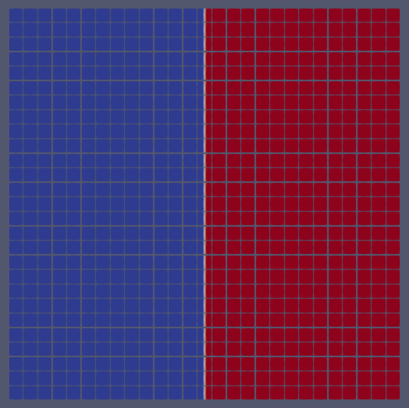
x. (Hint: The size and position of your domain can be found in the configuration file.)Qoutside, set the velocities and the bathymetry to be equal to 0, and the water height to 1.0 everywhere.BTimesDeltaQ to 0 for all its components, after all we do not need an NCP here, do we?The initial conditions should look like this:
If you get stuck or have a typo you cannot quite find, you can find an example solution at:
So, now that you hopefully have a working simulation we have to admit something. When we described the shallow-water equations to you, we sort of lied. Well not really, it's just that the equation above is the form of the SWE without bathymetry. With bathymetry, it looks as follows (note that the gravity term was moved from the flux to the NCP):
\( \begin{equation*} \label{SWE_w} \frac{\partial}{\partial t}\left( \begin{array}{lr} h \\ h u_1 \\ h u_2 \\ b \end{array} \right) + \nabla \underbrace{\begin{pmatrix} h u_1 & h u_2 \\ h u_1^2 & h u_1 u_2 \\ h u_2 u_1 & h u_2^2 \\ 0 & 0 \end{pmatrix}}_{ flux } + \underbrace{\begin{pmatrix} 0 & 0\\ h g*\partial_x(b+h) & 0\\ 0 & h g*\partial_y(b+h) \\ 0 & 0 \end{pmatrix}}_{ ncp } = \vec{0} \end{equation*} \)
Let's modify our implementation to take this into account, and while we're at it change our scenario a little, and heck why not learn about mesh refinement too? Mesh refinement in ExaHyPE 2 is controlled via a so-called refinement criterion. Cells can be sub-divided into 3^d cells so long as this would not cause the sub-cells to be smaller than the lowest cell size as defined in the configuration.
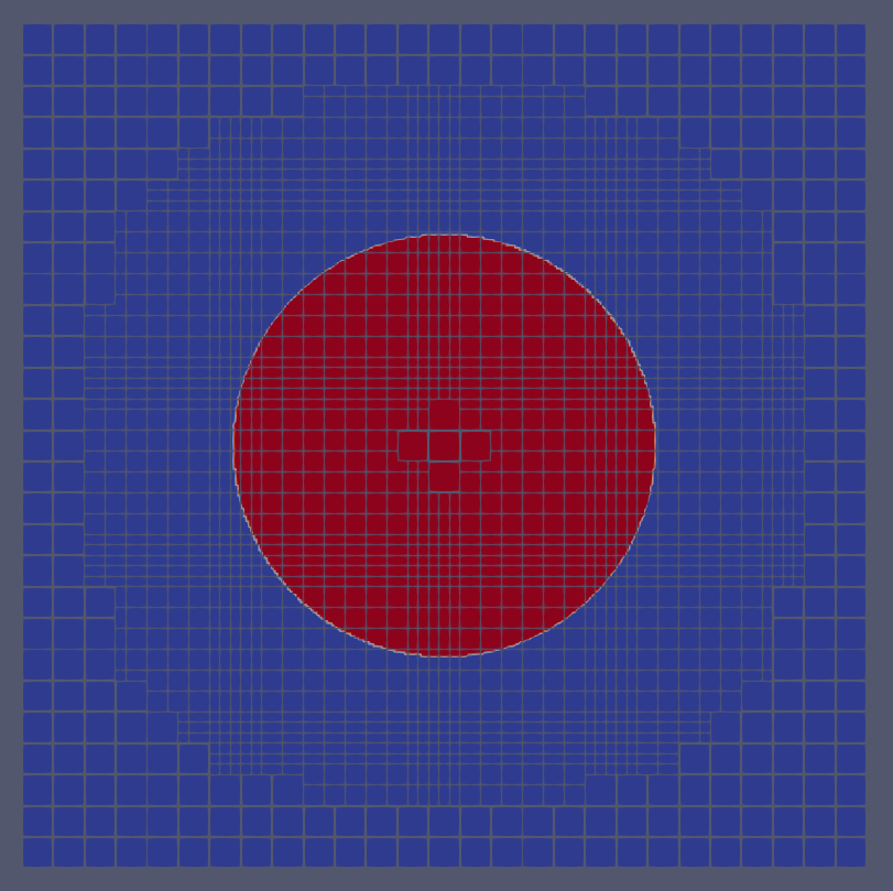
BTimesDeltaQ, and depends on the gradients of the values, which are stored in the parameter deltaQ. (Note that deltaQ is the finite difference in each normal direction)tarch::la::norm2() to compute the norm of a vector)refinementCriterion within your implementation file which currently always returns exahype2::RefinementCommand::Keep. Conditionally set it to return exahype2::RefinementCommand::Refine if within a distance of 0.3 to 0.7 of the center of the domain. With this, re-compile the project, and run it one final time.The initial conditions should look like this:
And once you are finished with these tasks, you can move on to The Euler Equations and Air Flow Over a Symmetric Airfoil, where you will build your own application from scratch.
If you get stuck or have a typo you cannot quite find, you can find an example solution at: