The Euler Equations and Air Flow Over a Symmetric Airfoil

New exercise, new equation! This time we will be simulating the euler equations, which approximate the flow of non-viscous fluids, but do take into account pressure differentials. In two dimensions, these take following form:

\(\begin{equation*} \label{Euler_equation} \frac{\partial}{\partial t}\left( \begin{array}{lr} \rho \\ \rho u_1 \\ \rho u_2 \\ E_t \end{array} \right) + \nabla \begin{pmatrix} \rho u_1 & \rho u_2\\ \rho u_1^2 + p & \rho u_1 u_2 \\ \rho u_2 u_1 & \rho u_2^2 + p \\ (E_t + p) u_1 & (E_t + p) u_2 \end{pmatrix} = \vec{0} \end{equation*} \)

The eigenvalues of the 2 dimensional euler equation are:

\(\begin{equation*} \left( \begin{array}{lr} \lambda_1 \\ \lambda_2 \\ \lambda_3 \end{array} \right) = \left( \begin{array}{lr} u - c \\ u \\ u + c \end{array} \right) \end{equation*} \)

We've also made use of two variables, the speed of sound in a medium c is defined as: \(\begin{equation} c = \sqrt{\frac{\gamma p}{\rho} } \end{equation} \)

And the pressure p can, for an ideal gas, be computed as: \(\begin{equation} p = (\gamma - 1) (E - \frac{\rho}{2} (u_1^2 + u_2^2) ) \end{equation} \) (Hint: this uses velocities u, not the momenta in either direction as the equation does)

Finally, \( \gamma \) is the ratio of specific heats, which here we choose as 1.4, corresponding to that of dry air at room temperature.

We have not provided you with a configuration file, so you will need to make your own. However since the Euler equations and the scenario we will attempt next are somewhat more unstable than the previous two (and also just to show of the features of ExaHyPE 2) we will use a different solver. This time, we will use a Finite Volumes solver. This can be created in the configuration as follows:

my_solver = exahype2.solvers.fv.godunov.GlobalAdaptiveTimeStep(
    name                  = "EulerSolver",
    patch_size            = 22,
    min_volume_h          = min_h,
    max_volume_h          = max_h,
    time_step_relaxation  = 0.5,
    unknowns              = unknowns,
    auxiliary_variables   = auxiliary_variables
)

This configuration is similar to that of the ADER-DG solver, obviously. The only parameter that we haven't encountered so far is patch_size, this controls the number of finite volumes which should be assembled together as one patch, i.e. which are solved at the same time. Here 22 means that there are 22 volumes per spatial dimension, so for a 2D problem this is 22x22=484 cells per patch.

• Exercises
  • First, create and fill a configuration file. Use a Finite Volumes solver for this, then set the domain size to 120x120, the offset to -10x-60 and the end-time to 10.0 . You can choose the mesh refinement of your choice, but we recommend a depth of 5 over the whole domain.
  • Once you are content with your configuration file, implement the flux and the eigenvalues for your solver.
  • Next, we will set the boundary conditions. These should be [1.0, 1.0, 0.0, 2.5]^T on the leftmost face of the domain. On all other faces, use absorbing boundary conditions. That is to say the values outside of the boundary should be equal to the values inside of the boundary.
  • Finally, we need to implement the initial conditions. We will try to simulate airflow over a symmetrical NACA airfoil. Specifically we will choose airfoil NACA 0012. The half-thickness of the airfoil is defined by following equation: \( \begin{equation} y_t = 5*0.12* ( 0.2969*\sqrt{x_n} - 0.1260*x_n - 0.3516*x_n^2 + 0.2843*x_n^3 - 0.1104*x_n^4 ) \end{equation} \) where x_n is x/100. The initial conditions within the airfoil should be [1000, 1.0, 0.0, 2.5]^T, those outside of the airfoil should be [1.0, 1.0, 0.0, 2.5]^T. (Note: We have committed here what we in the business call a "not accurate cheaty fake result", there are many good ways to simulate what we want to simulate and this is not one of them. But this is easy and it'll make a nice picture if you did it right, so don't tell anyone.)
  • Compile and run! If you have done everything correctly, your initial conditions should look something like the picutre below, and you should see a so-called bow shock develop over time as the flow causes higher pressure in front of your airfoil and lower pressure behind it.
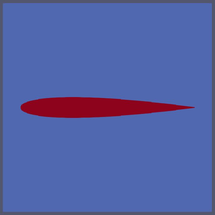
  • You are finished with all of the tasks we've prepared so you'll have to think up some more yourself, congratulations! Feel free to experiment some more, or go take a look in the applications folder to see what other people have done.

The initial conditions should look like this:

Solution

If you are stuck, you can look at the solutions over at:

• The Euler Equations and Air Flow Over a Symmetric Airfoil: Solution