Inheritance diagram for ComputeFirstDerivatives.ComputeFirstDerivativesFD4RK:

Collaboration diagram for ComputeFirstDerivatives.ComputeFirstDerivativesFD4RK:

Public Member Functions
def	__init__ (self, solver, is_enclave_solver)

def	user_should_modify_template (self)

def	get_includes (self)

def	get_body_of_operation (self, operation_name)

def	get_action_set_name (self)

Static Public Attributes
	ComputeDerivativesOverCell = jinja2.Template( + )

Private Member Functions
def	_add_action_set_entries_to_dictionary (self, d)

Private Attributes
	_solver

	_butcher_tableau

	_use_enclave_solver

Detailed Description

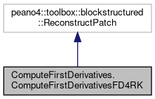
Explicit reconstruction of first derivatives for FD4 discretisation

FD4 is implemented as Runge-Kutta scheme. So we first have to recompute
the current solution guess according to the Butcher tableau. Then we feed
this reconstruction into the derivative computation. In theory, this is all
simple, but in practice things require more work.

We assume that developers follow @ref page_exahype_coupling "ExaHyPE's generic recommendation how to add additional traversals".
Yet, this is only half of the story. If they follow the vanilla blueprint
and plug into a step after the last time step

  if (repositories::isLastGridSweepOfTimeStep()
  and
  repositories::StepRepository::toStepEnum( peano4::parallel::Node::getInstance().getCurrentProgramStep() ) != repositories::StepRepository::Steps::AdditionalMeshTraversal
  ) {
    peano4::parallel::Node::getInstance().setNextProgramStep(
    repositories::StepRepository::toProgramStep( repositories::StepRepository::Steps::AdditionalMeshTraversal )
  );
  continueToSolve         = true;
}

then the reconstruction is only done after the last and final Runge-Kutta step. Alternatively, users might plug into the solver after each Runge-Kutta step. In principle, we might say "so what", as all the right-hand sides after the final step are there, so we can reconstruct the final solution. However, there are two pitfalls:

A solver might not hold the rhs estimates persistently in-between two time steps.
The solver's state always is toggled in startTimeStep() on the solver instance's class. Therefore, an additional grid sweep after the last Runge-Kutta sweep cannot be distinguished from an additional sweep after the whole time step. They are the same.

Consequently, we need special treatment for the very last Runge-Kutta step:

If we have an additional grid sweep after an intermediate RK step, we use the right-hand side estimate of \( \partial _t Q = F(Q) \) to store the outcome. Furthermore, we scale the derivative with 1/dt, as the linear combination of RK will later on multiple this estimate with dt again.
If we are in the very last grid sweep, we work with the current estimate.

The actual derviative calculation is "outsourced" to the routine

::exahype2::CellData  patchData( 
  oldQWithHalo, 
  marker.x(), marker.h(), 
  0.0, // timeStamp => not used here 
  0.0, // timeStepSize => not used here
  newQ 
);
::exahype2::fd::fd4::reconstruct_first_derivatives(
  patchData,
  {{NUMBER_OF_GRID_CELLS_PER_PATCH_PER_AXIS}},  // int                     numberOfGridCellsPerPatchPerAxis,
  {{HALO_SIZE}}, 
  {{NUMBER_OF_UNKNOWNS}},
  {{NUMBER_OF_AUXILIARY_VARIABLES}}
);

Wrapping up oldQWithHalo and newQ in a CellData object is a slight overkill (we could have done with only passing the two pointers, as we don't use the time step size or similar anyway), but we follow the general ExaHyPE pattern here - and in theory could rely on someone else later to deploy this to GPUs, e.g.

Right after the reconstruction, we have to project the outcome back again onto the faces. Here, we again have to take into account that we work with a Runge-Kutta scheme. The cell hosts N blocks of cell data for the N shots of Runge-Kutta. The reconstruction writes into the nth block according to the current step. Consequently, the projection also has to work with the nth block. exahype2.solvers.rkfd.actionsets.ProjectPatchOntoFaces provides all the logic for this, so we assume that users add this one to their script. As the present action set plugs into touchCellFirstTime() and the projection onto the faces plugs into touchCellLastTime(), the order is always correct no matter how you prioritise between the different action sets.

Further to the projection, we also have to roll over details. Again, exahype2.solvers.rkfd.actionsets.ProjectPatchOnto has more documentation on this.

Definition at line 10 of file ComputeFirstDerivatives.py.

Constructor & Destructor Documentation

◆ init()

def ComputeFirstDerivatives.ComputeFirstDerivativesFD4RK.__init__	(	self,
		solver,
		is_enclave_solver
	)

Definition at line 99 of file ComputeFirstDerivatives.py.

Member Function Documentation

◆ _add_action_set_entries_to_dictionary()

def ComputeFirstDerivatives.ComputeFirstDerivativesFD4RK._add_action_set_entries_to_dictionary	(	self,
		d
	)

private

    This is our plug-in point to alter the underlying dictionary

Definition at line 201 of file ComputeFirstDerivatives.py.

References ComputeFirstDerivatives.ComputeFirstDerivativesFD4RK._butcher_tableau, ComputeFirstDerivatives.ComputeFirstDerivativesFD4RK._solver, coupling.actionsets.AbstractLimiterActionSet.AbstractLimiterActionSet._solver, and ComputeFirstDerivatives.ComputeFirstDerivativesFD4RK._use_enclave_solver.

Referenced by ComputeFirstDerivatives.ComputeFirstDerivativesFD4RK.get_body_of_operation().

Here is the caller graph for this function:

◆ get_action_set_name()

def ComputeFirstDerivatives.ComputeFirstDerivativesFD4RK.get_action_set_name ( self )

Definition at line 237 of file ComputeFirstDerivatives.py.

◆ get_body_of_operation()

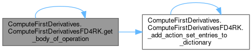
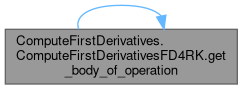
def ComputeFirstDerivatives.ComputeFirstDerivativesFD4RK.get_body_of_operation	(	self,
		operation_name
	)

Definition at line 228 of file ComputeFirstDerivatives.py.

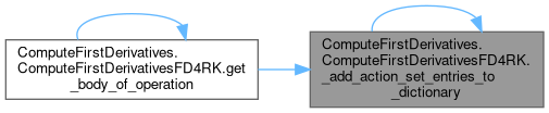
References ComputeFirstDerivatives.ComputeFirstDerivativesFD4RK._add_action_set_entries_to_dictionary(), and ComputeFirstDerivatives.ComputeFirstDerivativesFD4RK.ComputeDerivativesOverCell.

Here is the call graph for this function:

◆ get_includes()

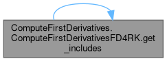
def ComputeFirstDerivatives.ComputeFirstDerivativesFD4RK.get_includes ( self )

Definition at line 194 of file ComputeFirstDerivatives.py.

◆ user_should_modify_template()

def ComputeFirstDerivatives.ComputeFirstDerivativesFD4RK.user_should_modify_template ( self )

Definition at line 190 of file ComputeFirstDerivatives.py.

Field Documentation

◆ _butcher_tableau

ComputeFirstDerivatives.ComputeFirstDerivativesFD4RK._butcher_tableau

private

Definition at line 110 of file ComputeFirstDerivatives.py.

Referenced by ComputeFirstDerivatives.ComputeFirstDerivativesFD4RK._add_action_set_entries_to_dictionary().

◆ _solver

ComputeFirstDerivatives.ComputeFirstDerivativesFD4RK._solver

private

Definition at line 109 of file ComputeFirstDerivatives.py.

Referenced by ComputeFirstDerivatives.ComputeFirstDerivativesFD4RK._add_action_set_entries_to_dictionary(), coupling.actionsets.SolveRiemannProblem.SolveRiemannProblem.get_body_of_operation(), coupling.actionsets.SpreadLimiterStatus.SpreadLimiterStatus.get_body_of_operation(), coupling.actionsets.VerifyTroubledness.VerifyTroubledness.get_body_of_operation(), coupling.actionsets.AbstractLimiterActionSet.AbstractLimiterActionSet.get_includes(), coupling.actionsets.SolveRiemannProblem.SolveRiemannProblem.get_includes(), and coupling.actionsets.VerifyTroubledness.VerifyTroubledness.get_includes().

◆ _use_enclave_solver

ComputeFirstDerivatives.ComputeFirstDerivativesFD4RK._use_enclave_solver

private

Definition at line 111 of file ComputeFirstDerivatives.py.

Referenced by ComputeFirstDerivatives.ComputeFirstDerivativesFD4RK._add_action_set_entries_to_dictionary().

◆ ComputeDerivativesOverCell

ComputeFirstDerivatives.ComputeFirstDerivativesFD4RK.ComputeDerivativesOverCell = jinja2.Template( + )

static

Definition at line 115 of file ComputeFirstDerivatives.py.

Referenced by ComputeFirstDerivatives.ComputeFirstDerivativesFD4RK.get_body_of_operation().

The documentation for this class was generated from the following file:

applications/exahype2/ccz4/ComputeFirstDerivatives.py

Public Member Functions

Static Public Attributes

Private Member Functions

Private Attributes

Detailed Description

Constructor & Destructor Documentation

◆ __init__()

Member Function Documentation

◆ _add_action_set_entries_to_dictionary()

◆ get_action_set_name()

◆ get_body_of_operation()

◆ get_includes()

◆ user_should_modify_template()

Field Documentation

◆ _butcher_tableau

◆ _solver

◆ _use_enclave_solver

◆ ComputeDerivativesOverCell

◆ init()