|
Peano
|
|
Peano
|
We have tree \( \mathcal{T} \) where each node has either 0 or \( k^d \) children, and \( k,d \in \{2,3\} \) are fixed constants. The level \( \ell(n) \) is the distance from the tree's root \( n_0 \) in graph. Let \( n_i \sqsubseteq_{\text{child of}} n_j, \ n_i,n_j \in \mathcal{T} \) denote that \( n_i \) is a child of \( n_j \), i.e. there's an edge from \( n_i \) to \( n_j \) and \( \ell (n_i) = \ell (n_j) + 1 \). Nodes \( \mathcal{T}_{leaves} = \{ n \in \mathcal{T}: \not \exists j: n_j \sqsubseteq_{\text{child of}} n \} \) are the leaves of the tree.
We also have a set \( \mathcal{P} = \{p_0, p_1, \ldots, p_{N_{comp}-1} \} \) of compute resources. Let \( C: \mathcal{T} \mapsto \mathcal{P} \) assign each tree node to a compute resource.
There is only one operation available: \( split(p_i, p_j, n, N) \) operates on \( \{ n_k: C(n_k)=p_i \} \neq \emptyset \) and \( \{ n_l: C(n_l)=p_j \} = \emptyset \). It takes \( n \leq \hat n \) leaf nodes assigned to \( p_i \) and assigns them to \( p_j \). Hereby, \( \hat n \) is the number of leaf nodes associated to \( p_i \). The split consequently might also reassign some non-leaf nodes. \( N \) is the total size of the current tree. The movement of the non-leaf nodes must following the tree topology: if the parent and at least one child of a node are both associated to \( p_i \), then this non-leaf node must be associated to \( p_i \) as well.
W.l.g. we may assume that the root \( n_0 \) is originally assigned to the first available compute resource: \( C(n_0) = p_0 \).
Notice we can not merge subtrees, i.e., split is not allowed to operate if \( \{ n_l: C(n_l)=p_j \} \neq \emptyset \). The splitted subtree can continue to construct to following levels without any further cost (see next section, and the example section).
The tree is not constructed in one rush. It originally consists solely of the root node. After that, we add one more level per step. After \( \ell_{max} \) steps, the tree is complete. We build it up level by level.
The \( \ell_{max} \) is known a priori. So is a \( \ell_{min} \) which is the minimal distance from any leaf node, i.e. unrefined node to the tree's root in the final tree. Throughout the grid construction, \( \ell < \ell_{max} \) is admissible for an unrefined node, and even \( \ell < \ell_{min} \leq \ell_{max} \) will occur early throughout the mesh construction. Once the tree construction has terminated, we however guarantee \( \ell_{min} \leq \ell(n) \leq \ell_{max} \) for each leaf.
By default, any new node that is added to the tree is assigned to the compute entity its parent has been assigned to. \( n_i, n_j \in \mathcal{T}: \ n_i \sqsubseteq_{\text{child of}} n_j \Rightarrow C(n_i) = C(n_j) \). Only the slits can change this transition afterwards. Without any split operations, the whole tree would eventually be associated to the root's compute resource \( C(n_0) = p_0 \).
Due to a sequence of split calls, we want to construct a mapping \( C \), such that
\( \forall p_i,p_j: \ \mathcal{T}_{leaves}(p_i) \approx \mathcal{T}_{leaves}(p_i) \)
where \( \mathcal{T}_{leaves}(p) = \{ n \in \mathcal{T}_{leaves}: C(n)=p \} \). We want to have a well-balanced assignment of leaves to processing units. The \( \approx \) sign is used, as we work with integers and hence cannot ensure exact equality. We might also be willing to accept a small, fixed deterioration from the optimum.
For a more advance metric of measuring the quality of the splitting, we introduce the splitting quality score \( w=C_2 \cdot \text{SplitCost}+C_1 \cdot \text{Imbalance} \), where \( \text{SplitCost}=\sum F(split(...)) \) is the sum up of costmetric output for every split operation (see next section), and \( \text{Imbalance}=MAX(\mathcal{T}_{leaves}(p_i)+C_3 \text{Surface}(p_i)) - MIN(\mathcal{T}_{leaves}(p_i)+C_3 \text{Surface}(p_i)) \). \(\text{Surface}(p_i)\) is the spatial boundaries for the subtree associated with \( p_i \), as the tree represents an adaptive refinement of a spatial domain. The smaller the quality score is, the better the splitting algorithm is.
In the current problem, \( C_3 \ll 1 \). i.e., for now, we do not care too much about the surface size as long as all leaves are spatially connected. For online problem where we do not know the tree structure in advance, We also set \( C_2 \ll C_1 \) (holds even for the superlinear model of splitting cost), i.e., the balance among compute resources is the top priority. For offline problem it does not hold anymore and we would like a low-cost spliting process as well.
This challenge in principle is very simple: We take the whole tree, count the number of leaves and issue a series of splitting calls. However, we want to make the splitting as cheap as possible: There is a cost function \( F( split(p_i, p_j, n, N) ) \) which depend on both in the number \( n \) (the number of leaves moved) and \( N \) (toal size of current tree). Due to the cost function, it consequently might be reasonable to issue splits while the tree is constructed and not at the very end, where \( N \) would become rather big.
In online problem, unfortunately, we do not know what the tree eventually will look like. We have guarantees regarding the minimum and maximum level of each node, but no further domain knowledge. On the other hand, in offline problem we know the complete structure of the tree, thus make lives much easier. Conclusively, the development of an "optimal" splitting strategy is not straightforward. We permanently have to balance between an eager decision to split, which is cheap yet might introduce the wrong splits that we cannot undo later, or waiting for further information which might make future splits more accurate but excessively expensive.
An offline problem means that we first construct the tree once without any splitting. And then restart from the beginning to do the split with the information of the whole tree. It can avoid the biggest problem in the online version: we can not make clever decisions as we know nothing about the future. Achieving low imbalance is easy in this case, and thus, the leading measure of split quality would be split cost. Several important remarks for the offline version of splitting:
The example section below can be helpful in understanding the offline splitting further.
The topology over \( \mathcal{P} \) is a tree topology in itself, i.e. the way how we split the tree introduces a tree topology over the individual compute entities.
In reality, the set \( \mathcal{P} \) is hierarchical in itself, i.e. it is actually a \( \mathcal{P} = \{ p_{0,0}, p_{0,1}, \ldots, p_{0,N_{cores}-1}, p_{1,0}, p_{1,1}, \ldots, p_{N_{nodes}-1,0}, \ldots, p_{N_{nodes}-1,N_{cores}-1} \} \). A good partition minimises
\( n_i \sqsubseteq_{\text{child of}} n_j \ \text{with} \ C(n_i)=p_{a,b} \wedge C(n_j)=p_{c,d}: a \not= c \)
In the outline challenge, all leaves are considered to have the same weight. However, it is possible that we introduce weights for each individual (interior) node.
The notion of leaves changes over time: As we build up the tree level by level, a node that has been a leaf at one point (and did feed into a split's cost function at this point) might become refined later on. While we do not know, in general, what the tree will look like, a lot of problems can provide indicators (it is likely that we'll refine up to a level \( \ell \geq \ell _{\text{min}} \) in this area) and consequently can assign a tree node which eventually becomes a refined one a weight that's bigger than other nodes. A lot of application codes can map their domain-specific knowledge about what the tree might look like onto a non-uniform cost metric.
In the vanilla version of the code, we assume that the tree is built up level-by-level. While the underlying simulation code constructs the tree in this way at the moment, we can alter the code such that the splitting algorithm decides where the tree is allowed to refine in the next step.
It is not clear if such a degree of freedom is of any use, but in principle it allows an algorithm to query more information about the tree before it continues, i.e. it can hold back with splitting decisions and instead tell the algorithm to continue to construct the tree (in certain areas) before it comes to its next decision.
We provide an example of (online) tree splitting. Below is a tree of four levels, where only the first nodes on levels 1 and 2 have children. The tree is constructed level by level, going through stages (I) to (IV). As we only have the split operation, the three good two-split candidates can be
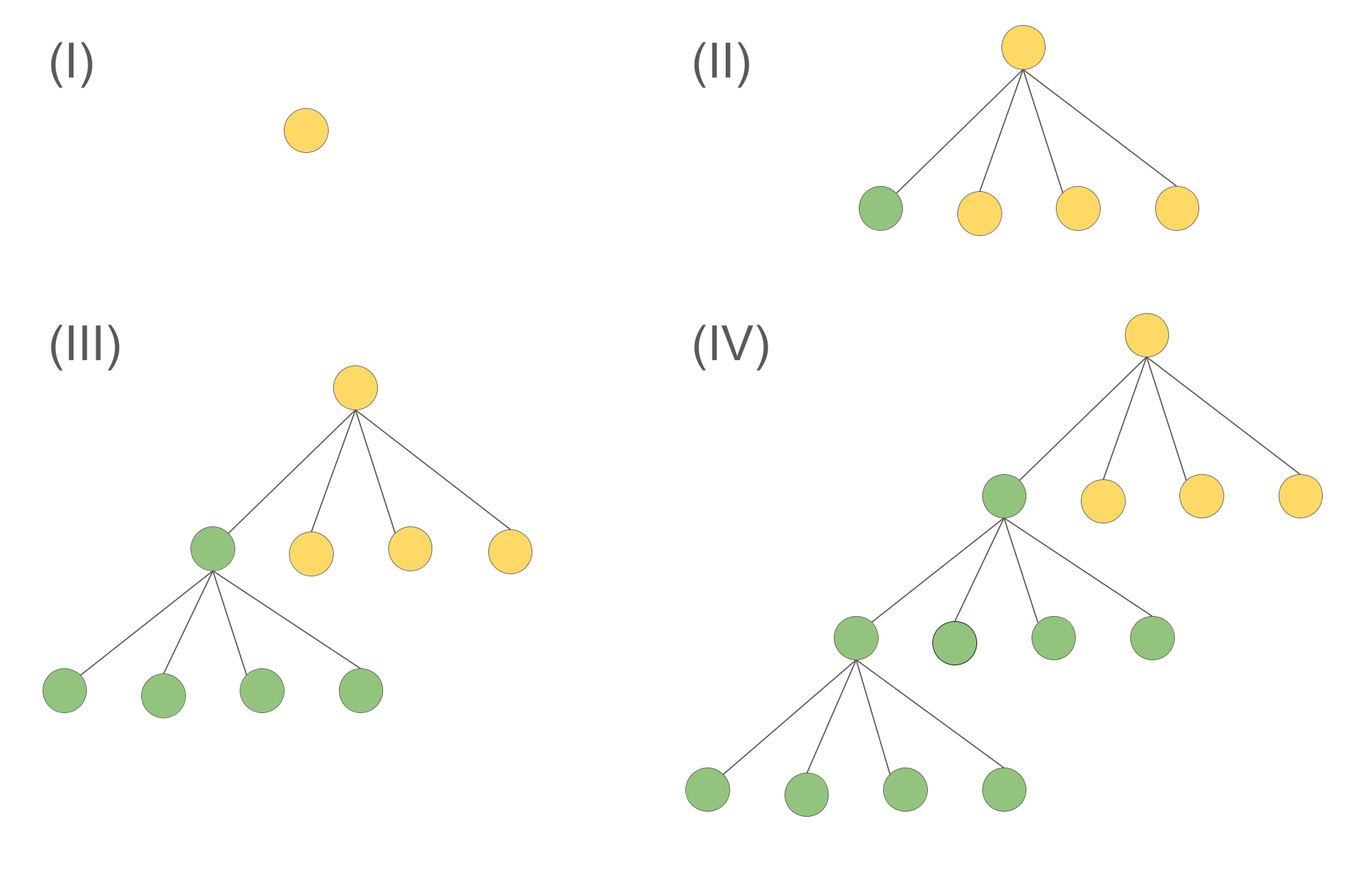
(1) split the first node in stage (II) to the second tree and finish the following construct. The imbalancing would be \( |7C_1-3C_1|=4C_1 \) (omit the surface term), with a split cost of \( C_2(A_1 + 4A_2) \) (assuming linear costmetric). The total quality score would be \( 4C_1+C_2(A_1 + 4A_2) \) (the smaller the better).
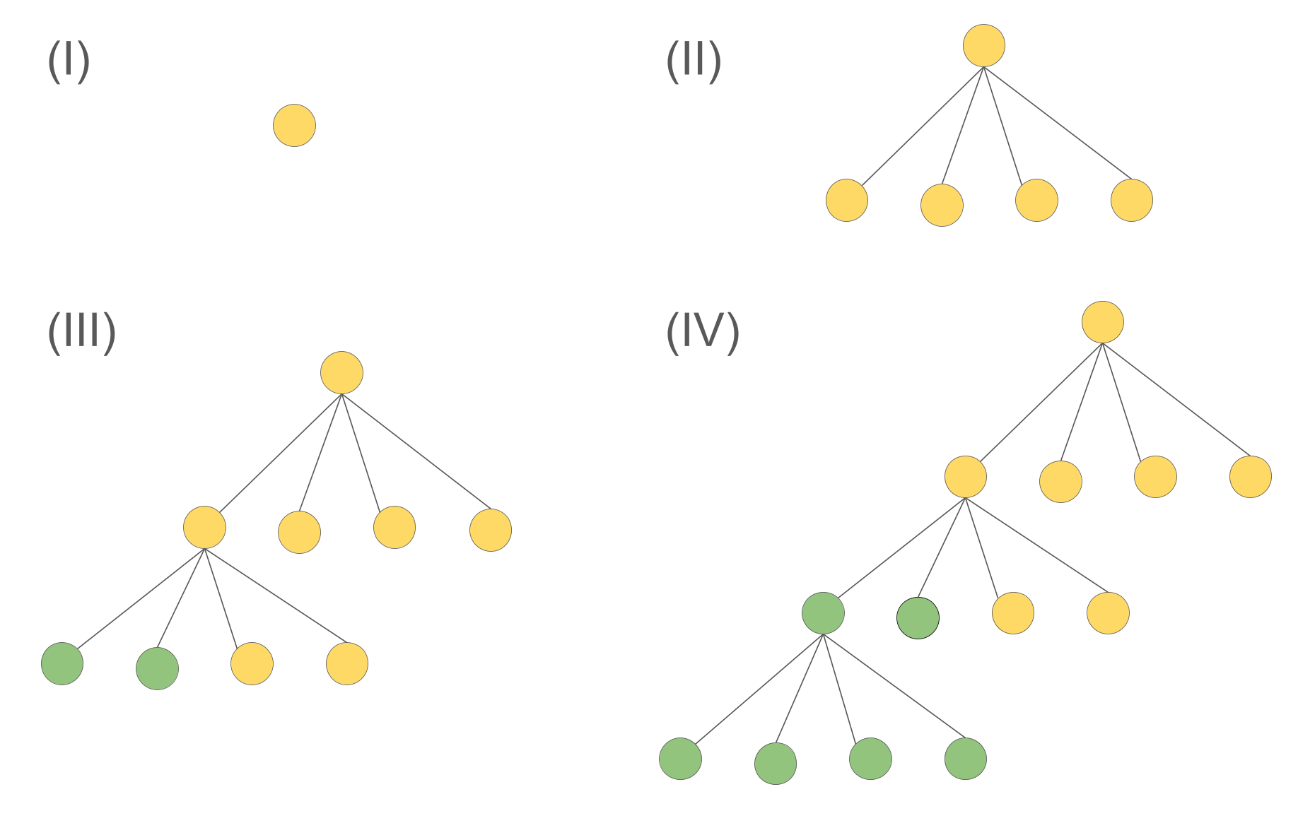
(2) split the first two nodes in stage (III) to the second tree and finish the following construct. The imbalancing would be \( |5C_1-5C_1|=0 \), with a split cost of \( C_2(2A_1 + 7A_2) \). The total quality score would be \( 2C_2(2A_1 + 7A_2) \).
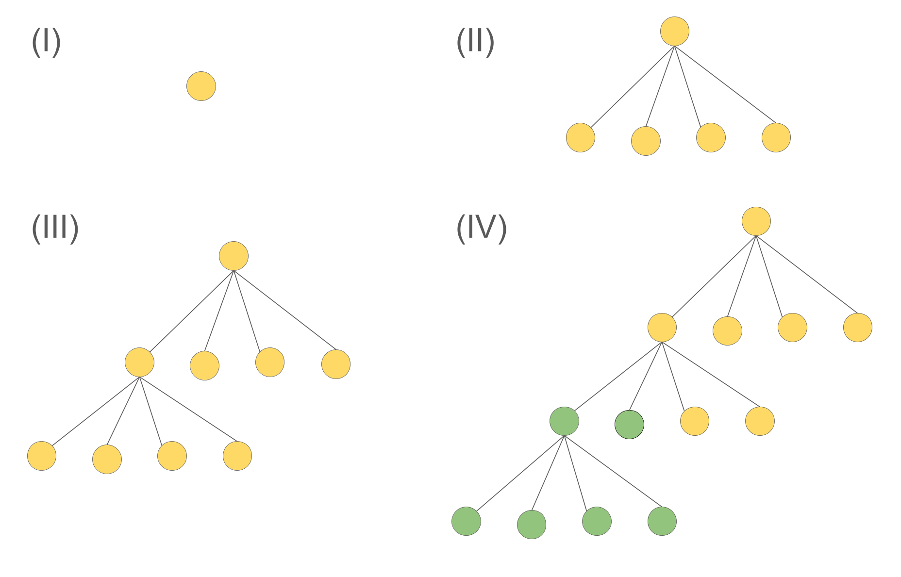
(3) Split the first two nodes on level 2 and all in level 3 in stage (IV) to the second tree. The imbalance would be \( |5C_1-5C_1|=0 \), with a split cost of \( C_2(5A_1 + 10A_2) \) (number of leaves moved). The total quality score would be \( C_2(5A_1 + 10A_2) \).
It is quite clear that option (1) is not good as it chooses an early, aggressive tree splitting, though the splitting cost is cheap, the heavy imbalance indicates it is not a good strategy. Comparing options (2) and (3) is a little more tricky: (2) has a smaller score, however, it has to "foresee" that the first node is going to be refined to make this clever decision. (3), on the other hand, does not have this issue, as at stage (IV) the tree has been constructed completely. Of course, it then has to pay the price for moving more nodes in the split operation.
To summarise, option (1) is not acceptable, option (3) is acceptable but expensive, and option (2) is best but requires a clever splitting strategy. For the corresponding offline version of this example, (3) is quite easy to find and we hope a good algorhitm to find (2) efficiently. It is more practical in offline version because we do know the future at stage (III) in this case.
Here we provide a example of splitting on the same tree, but now triple splitting from an offline problem prespective.
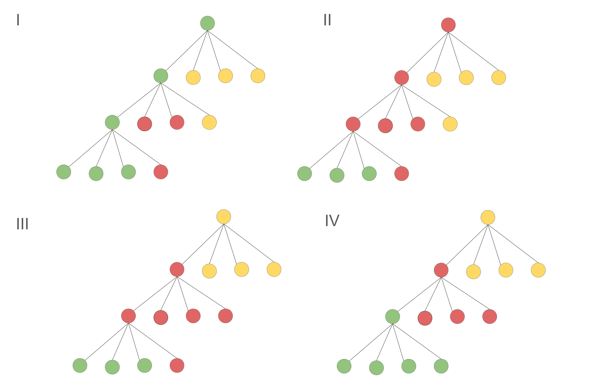
There are multiple ways to split the tree with minimum leaf imbalance (again we drop surface term), which is \( 3:3:4 \). However they are from different splitting processes:
It is obvious (4) have the lowest cost of splitting, and it is because it makes better split decisions at early stage of tree construction, while keep the leaves imbalance unchanged. Now the problem is: given the structure of an arbitrary tree, can we find an algorithm to find the good splitting like (4)?