ExaHyPE's Finite Volume scheme is based upon block-structured Cartesian meshes. All Finite Volume solvers work with blockstructured AMR: They embed \( p \times p\) patches into the octants (cells of the spacetree). To avoid confusion, I prefer to use the term volume for the cells within the patch, as cell would be ambigous given that we construct the host mesh from spacetree cells.

With the Finite Volume methods, we only have single-shot methods at the moment. That is, Peano runs over the octants of the mesh, i.e. the patches. Per patch, it calls and ExaHyPE update kernel, which takes the patch and moves it forwards in time by a given \( \Delta t \). ExaHyPE is shipped with several update schemes. You can obviously also write your own numerical scheme manually, or you employ ExaHyPE's kernel domain-specific language (DSL).

Storage scheme

Every patch has to depends upon its neighbouring, i.e. face-connected patches. To be able to do this, ExaHyPE passes a \( (p+2N)^d \) patch into a kernel, where \( p \) is the number of volumes per patch, \( d \) is the dimension, and \( N \geq 1 \) is halo size. Different Finite Volume schemes have different halo sizes. You may assume that ExaHyPE befills these halo values with valid data from the neighbours, i.e. their synchronisation is none of the kernel's business. The input is called \( Q_{in} \) from hereon. The kernel returns a \( (p+2 N)^d \) with the new time step's data, called \( Q_{out} \).

Here are some details about the data used within the kernels:

The halo data, i.e. the \( N \) layer around the patch is automatically befilled. However, we only maintain the face-connected data. Consequently, the diagonal (corners) do not exist. To make the whole logic easier, the \( Q_{in} \) nevertheless hold these data. They contain garbage. Example: In a \( 7 \times 7 \) patch world with \( N=2 \), we have 49 volumes in the core centre, surrounded by \( 2d \cdot (N \cdot p^{d-1}) = 4 \cdot (2 \cdot 7) \) face-connected values. The \( 4 \cdot (2 \cdot 2 ) \) corners of the halo do not hold any meaningful data. Nevertheless, we let \( Q_{in} \) holds a \( (7+2\cdot 2) \) volumes
The volumes within \( Q_{in} \) and \( Q_{out} \) are ordered lexicographically.
The data are stores as array of structs (AoS).
If a PDE is described by \( K_{pde} \) real values subject to the wave equations and \( K_{aux} \) auxiliary variables (material parameters), then the \( Q_{in} \) contains \( K_{pde} + K_{aux} \) values (degrees of freedom) per volume. The \( Q_{out} \) however contains only the \( K_{pde} + K_{aux} \) values, too, but the \( K_{aux} \) material parameters do not evolve in time and therefore are the same as in \( Q_{in} \).
Besides \( Q_{in} \) and \( Q_{out} \) a kernel is given the current time \( t \) and the time step size \( \Delta t \).
We never write a kernel for only one patch. We always write kernels that can advanced multiple patches in one go. So the "update one patch" is a special case.

Data structures

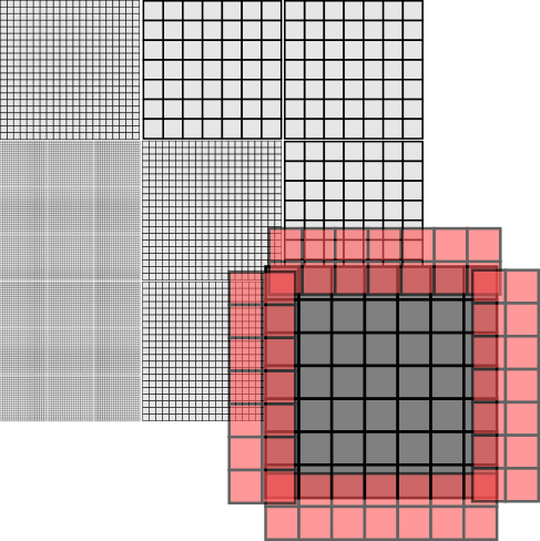
Each Finite Volume solver embeds \(N \times N\) patches into the octants (cells of the spacetree). ExaHyPE is built on top of Peano, and Peano realises a strict element-wise traversal, i.e. there's no way to access the neighbour cell of a cell directly. However, we can hijack the faces.

The idea here is that we embed a \( 2N\) \( (d = 2) \) or \(2N^2 \) \( (d=3) \), respectively, patches into each face. Let this auxiliary patch overlap the adjacent cells. Then, we effectively have a halo of one cell available within each cell: We know the cell data. We also have access to the \( 2d \) faces where each hosts a degenerated patch. One layer of this patch is a copy of our own data, i.e. does not give us additional information. The other layer of the auxiliary patch however holds data from the neighbour. It gives us information from the neighbour patch.

Keeping face and patch data consistent

Projecting the patches onto the face data structures and back is a mechanical task. Therefore, we offer a toolbox to relieve you from the pain to recode it over and over again. Using this toolbox, you add the projections to your algorithmic steps, and the API then automatically injects these features (aspects) into your code:

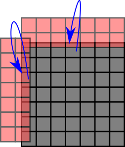
The image above illustrates what ProjectPatchOntoFaces does: It knows the dimensions of both the patches and the face auxiliary data structures and thus can ensure that the right data is copied from the cell into the \(2^d\) faces when we leave a cell throughout the grid traversal.

Augment patch with halo

The action set ReconstructPatchAndApplyFunctor works slighlty different yet can be read, from a patch projection point of view, as transpose of ProjectPatchOntoFaces: It creates a auxiliary variable reconstructedX with X being the name you gave the Unknowns of the patch. This auxiliary variable has the dimensions \(N+2 \times N+2 \times N+2\). It then copies over the patch data into this auxiliary patch and uses the faces to supplement it with halo data around it. So that it, you get the original patch data plus the cells around it in one big patch.

Code organisation

Peano offers a toolbox in toolbox::blockstructured which offers most of the basic data structures and action sets. The actual patches can either be embedded as plain arrays into each cell, or they can be held as arrays on the heap and the cells hold (smart) pointers to these heap objects. It depends on your use case which variant is faster.

On the Python API side, the class exahype2.solvers.fv.FV is the base class of all Finite Volume solvers. Its class documentation holds a lot of background information on the solver design and data flows. There are two major subclasses: exahype2.solvers.fv.SingleSweep and exahype2.solvers.fv.EnclaveTasking. They realise a straightforward realisation with one mesh traversal per time step or the enclave concept, respectively.

Implementation

Our discussion of an implementation of the scheme - which can be read as blueprint of our compute kernels in ExaHyPE - is inspired by

@article{10.1145/3406835,
author = {Uphoff, Carsten and Bader, Michael},
title = {Yet Another Tensor Toolbox for Discontinuous Galerkin Methods and Other Applications},
year = {2020},
issue_date = {December 2020},
publisher = {Association for Computing Machinery},
address = {New York, NY, USA},
volume = {46},
number = {4},
issn = {0098-3500},
url = {https://doi.org/10.1145/3406835},
doi = {10.1145/3406835},
abstract = {The numerical solution of partial differential equations is at the heart of many grand challenges in supercomputing. Solvers based on high-order discontinuous Galerkin (DG) discretisation have been shown to scale on large supercomputers with excellent performance and efficiency if the implementation exploits all levels of parallelism and is tailored to the specific architecture. However, every year new supercomputers emerge and the list of hardware-specific considerations grows simultaneously with the list of desired features in a DG code. Thus, we believe that a sustainable DG code needs an abstraction layer to implement the numerical scheme in a suitable language. We explore the possibility to abstract the numerical scheme as small tensor operations, describe them in a domain-specific language (DSL) resembling the Einstein notation, and to map them to small General Matrix-Matrix Multiplication routines. The compiler for our DSL implements classic optimisations that are used for large tensor contractions, and we present novel optimisation techniques such as equivalent sparsity patterns and optimal index permutations for temporary tensors. Our application examples, which include the earthquake simulation software SeisSol, show that the generated kernels achieve over 50\% peak performance of a recent 48-core Skylake system while the DSL considerably simplifies the implementation.},
journal = {ACM Trans. Math. Softw.},
month = oct,
articleno = {34},
numpages = {40},
keywords = {ADER-DG, Tensor operations, finite element method, high-performance computing}
}

who write down the algorithm as a sequence of tensor multiplications, i.e. generalised matrix-matrix equations. This does not work in ExaHyPE 1:1 as we support non-linear PDEs in the generic kernel formulations. However, we can use similar operator concatenation ideas.

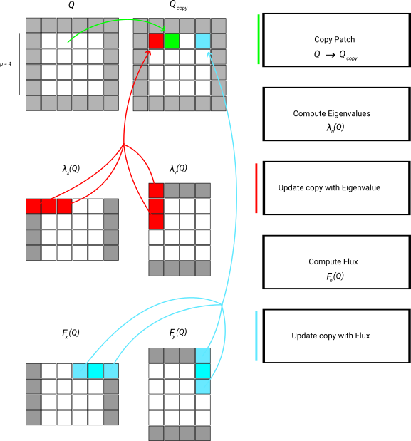
We demonstate the data flow by means of the simplified numerical flux which only takes the average. This algorithm consists of a strict sequence of steps:

We evaluate \( S(Q) \) per voxel. The output is stored in a \( p \times p \times p \) patch where each volume holds \( K_{pde} \) values. The output is called \( Q_{S} \).
We evaluate \( F(Q)_x \) per voxel. That the flux in one direction. The output is stored in a \( (p+2N) \times p \times p \) patch where each volume holds \( K_{pde} \) values. The output is called \( Q_{F_x} \). Note that this is the core patch extended by the halo in one direction!
We evaluate \( F(Q)_y \) per voxel. That the flux in one direction. The output is stored in a \( p \times (p+2N) \times p \) patch where each volume holds \( K_{pde} \) values. The output is called \( Q_{F_y} \). Note that this is the core patch extended by the halo in one direction!
We evaluate \( F(Q)_z \) per voxel. That the flux in one direction. The output is stored in a \( p \times p \times (p+2N) \) patch where each volume holds \( K_{pde} \) values. The output is called \( Q_{F_z} \). Note that this is the core patch extended by the halo in one direction!

Now all temporary data are available. We prepare the output and then add the PDE contributions. This part is basically a stencil variant. Or we can write it down as a tensor-vector product which is added to \( Q_{out} \):

We copy over \( Q_{in} \) into \( Q_{out} \). Per voxel, we have o copy \( K_{pde} + K_{aux} \) unknowns.
Add to each voxel \( Q_{in}[x,y,z] \) the value \( \Delta t \cdot Q_{S}[x,y,z] \). This loop runs over \( K_{pde} \) unknowns only. The \( K_{aux} \) entries are not touched.
Add to each voxel \( Q_{in}[x,y,z] \) the value \( \frac{\Delta t}{2h} \cdot (Q_{F_x}[x-1,y,z]+Q_{F_x}[x,y,z]+Q_{F_x}[x,y,z]+Q_{F_x}[x+1,y,z])\). This loop runs over \( K_{pde} \) unknowns only. The \( K_{aux} \) entries are not touched.
Add to each voxel \( Q_{in}[x,y,z] \) the value \( \frac{\Delta t}{2h} \cdot (Q_{F_y}[x,y-1,z]+2Q_{F_y}[x,y,z]+Q_{F_y}[x,y+1,z])\). This loop runs over \( K_{pde} \) unknowns only. The \( K_{aux} \) entries are not touched.
Add to each voxel \( Q_{in}[x,y,z] \) the value \( \frac{\Delta t}{2h} \cdot (Q_{F_z}[x,y,z-1]+2Q_{F_z}[x,y,z]+Q_{F_z}[x,y,z+1])\). This loop runs over \( K_{pde} \) unknowns only. The \( K_{aux} \) entries are not touched.

The extension to Rusanov for example is straightforward, as long as we take into account that our "stencil" here has to incorporate the max function. Below is schematic illustration of the data flow:

Note that the scheme as well as the description lack an important detail: Every single step is to be done over a set of patches, as we update multiple patches in one go. In the kernels, we can write down this logic as a sequence of operators, but once you employ our xDSL kernel language, the underlying kernel generator will permute and fuse all the loops and operations.