If you want to solve systems of PDEs where some PDEs advance on different time scales, solve different problems, are active in different domains, and so forth, you have two options on the table: You can model the solvers as one big system or you can logically code the solvers as two totally separate things and couple them.

If you have to run some postprocessing, you also have two options: Either make the postprocessing a "real" postprocessing by adding it as postprocessing step to your solvers of choice, or you add separate mesh sweeps which perform the postprocessing.

The former version is faster, as you read/write data only once and you do not impose additional mesh traversals. The latter version is the way to go if you need some boundary exchange prior such that halos, for example, are up-to-date. It might also be appropriate if you want to couple the hyperbolic solvers to other solvers, such as an elliptic term or a solid in a fluid-structure interaction scenario. When it comes to the coupling of two solvers, the first approach sketched is simple: If the two solvers feature \( N_1 \) and \( N_2 \) unknowns, you simply create one new solver with \( N_1+N_2 \) unknowns and you provide flux functionsm, ncps, ...for all of the components. The big disadvantage of this approach is that all solvers have to advance in time at the same speed, that you might replicate code if you have already two existing solvers, and that you also might run a lot of unneeded calculations if only some PDE equations evolve actually in time. Technically, the implementation of this variant however is straightforward and we will not discuss it further here, i.e. our description from hereon assumes that you work with two solvers and/or separate mesh sweeps.

Using multiple solvers within ExaHyPE is, in principle, straightforward, too. You create two solver instances and you add them to your project. Both solvers then will be embedded into the mesh and run independently. They will hence interact through the adaptive mesh refinement - if one solver refines, the other one will follow - but otherwise be totally independent. While this approach allows us to have a clear separation-of-solvers, the coupling of the two systems is not that straightforward. And we have to couple them if we want to solver our initial setup phrased as system of PDEs.

Preparing the PDEs to be coupled

How to couple the PDEs depends upon the fact if you want to directly project the solutions onto each other of if you make one PDE feed into the other one via the right-hand side (or in general some "material" parameters within its PDE other than the evolution unknowns). If you coupld PDEs directly, you can use your PDE solvers as they stand.

To prepare the system of PDEs in the other case, I recommend to add new material (auxiliary) parameters to each PDE which contain the cooupling term. That is, if you have two solver A and B and B has an impact on A through a scalar and A influences B through a vector, thend you add one material parameter to A and three to B.

Those material parameters are not material parameters in the traditional sense. They change over time. B will set the material parameters of A and vice versa.

Coupling the solution data

There are two places where we can add coupling, i.e. map solution data onto each other: It can either be a preprocessing step of the time step or a postprocessing step. While, in principle, both approaches do work here, there's a delicate difference: In the pre-processing step, we have access to the patch data plus the halo. In the post-processing step, we have only access to the patch content.

We note that we exclusively discuss volumetric mapping in this section. This is the only coupling we support at the moment within ExaHyPE, i.e. we do not support mapping of face data onto each other (anymore). Besides volumetric coupling, you can obviously "only" couple global properties with each other. This is however similar to the time step synchronisation as discussed below and therefore not subject of further discussion.

Coupling the time step sizes

Unless you use fixed time stepping schemes with hard-coded time step sizes that match, any two solvers with ExaHyPE run at their own speed. Even more, each individual cell runs at its own speed and hosts its own time stamp. For local timestepping, different cells may advance at different speed in time. For adaptive timestepping, all cells of one solver will advance with the same time step size.

For most solvers, it is therefore sufficient to plug into getAdmissibleTimeStepSize() of the superclass. Overwrite it, call the superclass' variant and then alter the returned value.

class mynamespace::MySolver: public MyBaseClass {
  ... 
  getAdmissibleTimeStepSize() const override;
};
 
 
 
#include "repositories/SolverRepository.h"
 
double mynamespace::MySolvergetAdmissibleTimeStepSize() const {
  // get vanilla version of time step size, i.e. only the one computed
  // by our solver
  double myTimeStepSize = MyBaseClass::getAdmissibleTimeStepSize();
  double otherTimeStepSize = repositories::MyOtherSolver.getAdmissibleTimeStepSize();
  
  // now we combine it with each other and return result
} 

This is the approach used in Euler example with self-gravitation via the Poisson equation. If you want to use local time stepping or run checks on the timestamp per cell, you will have to alter the cell's meta data holding its time stamp. Things in this case become more involved, i.e. you will have to study the underlying action sets and change the generated source code in there.

Localisation

ExaHyPE couples volumetrically. That does not mean that all solvers have to be solved everywhere. Indeed, the idea to offer support for multiple solvers arose originally from the a posteriori limiting of Dumbser et al where a Finite Volume solver complements ADER-DG solutions where shocks arise.

Most projects that follow these rationale realise the same pattern: We define two different solvers, and we couple them with each other. The coupling (and solve) however are local operations:

The low-order (typically Finite Volume - we therefore always refer to Finite Volumes or FV from hereon) solver is our fallback strategy and we therefore neither solve with Finite Volumes everywhere in the computational domain nor should do we store the corresponding data.
The higher-order scheme is used everywhere where the FV is not applied or labelled as valid.
The FV and the higher-order solver are not coupled everywhere but only in boundary regions.

We will effectively end up with a domain decomposition where parts of the computational domain are handled by the higher-order solver and the other parts are handled with FV. To realise this, we need a marker or oracle, i.e. a magic function per cell which tells us, similar to a multi-phase flow, which solver rules in this particular cell. The marker will guide us which solver is "valid" in which cell, where one solver overrules the other one, and where we do not have to store one solver's data or the other.

The image below illustrates the core idea behind typically coupling approaches in ExaHyPE. The sizes of the overlap might differ, but the principle is always the same. The illustration shows the minimal overlap that we can typically use. Both the upper and the lower mesh illustrate the same mesh. I use colours to show which solver exists in which mesh cell.

Solver A is running within the filled cells visualised on the the top. In empty cells, A neither solves anything nor does it hold data.
Solver B is running within the filled cells visualised on the bottom. In empty cells, B neither solves anything nor does it hold data.
Consequently, dark red cells are exclusively solved by A, whereas dark green cells are exclusively B.
In orange cells, A solves its PDE. Afterwards, A's updated solution is projected onto B's solution. That is, the blue cells hold B's data, but they are not updated by B but instead hold projections of A's data. They kind of serve as boundary layer for B.
In the yellow cells, A does not solve its PDE but holds A's data. After each step, the cell's solution by B (light green) is written into A's data. The yellow cells serve as Dirichlet boundary data for A's solve.

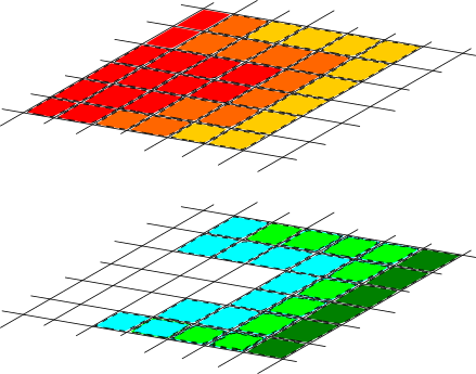
Starting from this description, sophisticated coupling equations can be realised, where you exploit the fact that we have a volumetric overlap.

Localisation guided by a marker

Skip this section if you prefer a hard-coded marking of active regions.

Avoid that solver data is held everywhere

Once you know where a solver is valid, it makes sense also to only store the solver's data in the valid region. Otherwise, a lot of memory is "wasted" which furthermore will be moved/accessed in each and every grid sweep, as the mesh management of Peano so far does not know that ExaHyPE might not need the data. ExaHyPE has to let Peano know.

The technical principles behind such a localisation are discussed on a generic Peano page of its own. ExaHyPE builds up pretty deep inheritance hierarchy where every subclass specialises and augments the basic numerical scheme, and also implements additional guards when data is stored or not. However, most of these subclasses rely on only six routines to control the data flow:

_provide_cell_data_to_compute_kernels_default_guard(),
_load_cell_data_default_guard(),
_store_cell_data_default_guard(),
_provide_face_data_to_compute_kernels_default_guard(),
_load_face_data_default_guard(),
_store_face_data_default_guard(),

The implementation then uses these predicates to puzzle the actual storage scheme together via calls similar to

self._patch.generator.load_store_compute_flag = "::peano4::grid::constructLoadStoreComputeFlag({},{},{})".format(
    self._provide_cell_data_to_compute_kernels_default_guard(),
    self._load_cell_data_default_guard(),
    self._store_cell_data_default_guard(),
)

By default, most solvers only store data for unrefined cells. They mask coarser levels with in the tree out.
Subclasses such as enclave tasking variations augment the guards further such that not all data are stored all the time. Nothing stops you from adding further constraints and to use a solver only in a certain subdomain for example.

The actual solution coupling

For the actual solver coupling, four hook-in points are available:

The dedicated solver preprocessing action set.
The hook-in preprocess_reconstructed_patch, which injects code right before the actual compute kernel (Finite Volume scheme, e.g.) is triggered.
The hook-in postprocess_updated_patch, which injects code right after updated time-step data. This snippet is called after the compute kernel has terminated. For Runge-Kutta style solvers, aka multi-step solvers, there are two of these hook-ins: One called after every intermediate step and one called once we compute the final linear combination of these intermediate outcomes.
The dedicated solver postprocessing action set.

These steps all have differen properties. The global preprocessing precedes any solver routine, i.e. it is called before any compute kernel on any solver is launched. It also is guaranteed to run sequentially, i.e. there is nothing running in parallel to the preprocess actino set. For the postprocessing, similar arguments hold. These steps come after all solvers have updated their solution. The kernel hook-ins (2) and (3) in contrast can run in parallel.

Any coupling can be arbitrary complicated, but there are several off-the-shelf routines offered in toolbox::blockstructured. Interesting variants include toolbox::blockstructured::copyUnknown() and ::toolbox::blockstructured::computeGradientAndReturnMaxDifference(). Besides those guys, you might also want to use the AMR routines within the blockstructured toolbox and the ExaHyPE folders, where you find, for example, linear interpolation and restriction.

Important: If you couple two solvers, you have to carefully take into account

in which order these solvers run; If that makes a difference, you might want to use the dedicated post- and pre-processing action sets.
wheather or not you use enclave solvers. The later ones take the data out of the mesh after their primary sweep and insert it back into the mesh. This has to be taken into account when you interpolate: data might be extracted from the mesh and then be put back in;
if you localise a solver, i.e. store it only in some places, you will have garbage on faces around this localised area.

See also: toolbox/blockstructured/Copy.h; toolbox/blockstructured/Derivative.h; toolbox/blockstructured/Interpolation.h; toolbox/blockstructured/Restriction.h

Table of Contents