Two-dimensional Euler Equation

The Euler equation describe the movement of a fluid if there is neither loss of energy due to frictional forces nor heat conduction in the system. In the finite volume form and given no external forces, the two-dimensional form of the Euler equation appears as follows:

\( \frac{\partial}{\partial t}\left( \begin{array}{lr} \rho \\ \rho u_1 \\ \rho u_2 \\ E_t \end{array} \right) + \nabla \begin{pmatrix} \rho u_1 & \rho u_2\\ \rho u_1^2 + p & \rho u_1 u_2 \\ \rho u_2 u_1 & \rho u_2^2 + p \\ (E_t + p) u_1 & (E_t + p) u_2 \end{pmatrix} = \vec{0} \)

Where \( \rho \) is the density, u is the velocity, \( E_t \) is the energy and p is the pressure.

This can also be rewritten as

\( \frac{\partial}{\partial t} \begin{pmatrix} \rho\\j\\\ E \end{pmatrix} + \nabla\cdot\begin{pmatrix} {j}\\ \frac{1}{\rho}j\otimes j + p I \\ \frac{1}{\rho}j\,(E + p) \end{pmatrix} = \vec{0} \)

To implement this equation, the following things are needed: the initial condition, the boundary conditions, the maximal eigenvalue, the flux, and (optionally) the refinement criterion.

Initial Conditions

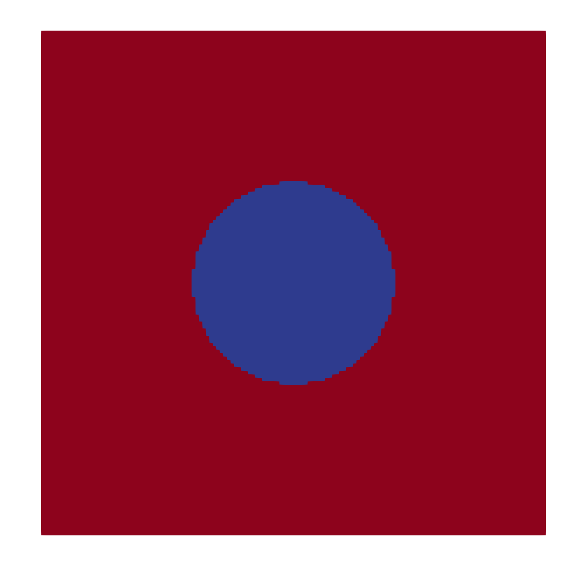
We start with the initial conditions: here we define a starting configuration with a uniform density of 1.0, a uniform starting momentum of 0.0 in both x- and y-directions and a starting energy that is 1.0 inside of a circle of radius 0.2 around the center of the domain and 1.01 outside of it. Note that we use momenta and not velocities as our variables of choice, this will affect the formulation of some of the equations later.

Boundary Conditions

Then we can define our boundary conditions. You can choose any boundary conditions you prefer but we have chosen to use the homogeneous Neumann boundary conditions.

Eigenvalues

Next, we can define the eigenvalues of our system. The eigenvalues of the 2-dimensional Euler equation are:

\( \left( \begin{array}{lr} \lambda_1 \\ \lambda_2 \\ \lambda_3 \end{array} \right) = \left( \begin{array}{lr} u - c \\ u \\ u + c \end{array} \right) \)

Where c is the wave propagation speed. For dry air, which can be approximated as an ideal gas, c depends on the pressure as follows:

\( \left( \begin{array}{lr} \gamma \\ p \\ c \end{array} \right) = \left( \begin{array}{lr} 1.4 \\ (\gamma - 1) ( E_t - \frac{1}{2 \rho} (\rho u)^2 ) \\ \sqrt[]{\frac{\gamma p}{\rho}} \end{array} \right) \)

Result

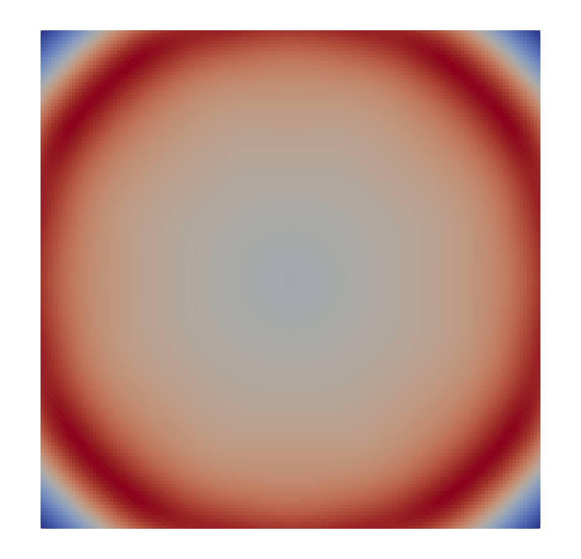
t=0.0 s

t=1.0 s

The computed energy of the 2D Euler equation at times t=0.0 s and t=1.0 s.

Three-dimensional Euler Equation

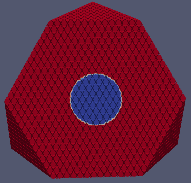
Finally, we can implement the Euler equation in three dimensions.

The three-dimensional Euler equation are very similar to the two-dimensional equations:

\( \frac{\partial}{\partial t}\left( \begin{array}{lr} \rho \\ \rho u_1 \\ \rho u_2 \\ \rho u_3 \\ E_t \end{array} \right) + \nabla \begin{pmatrix} \rho u_1 & \rho u_2 & \rho u_3\\ \rho u_1^2 + p & \rho u_1 u_2 & \rho u_1 u_3 \\ \rho u_2 u_1 & \rho u_2^2 + p & \rho u_2 u_3 \\ \rho u_3 u_1 & \rho u_3 u_2 + p & \rho u_3^2 + p \\ (E_t + p) u_1 & (E_t + p) u_2 & (E_t + p) u_3 \end{pmatrix} = \vec{0} \)

These have the same eigenvalues as the 2D solution:

\( \lambda = \left( \begin{array}{lr} u-c \\ u \\ u+c \\ \end{array} \right) \)

And you can use the same approximation for the pressure and wave velocity:

\( \left( \begin{array}{lr} \gamma \\ p \\ c \end{array} \right) = \left( \begin{array}{lr} 1.4 \\ (\gamma - 1) * ( E_t - \frac{\rho \|u\|}{2} ) \\ \sqrt[]{\frac{\gamma p}{\rho}} \\ \end{array} \right) \)

Result

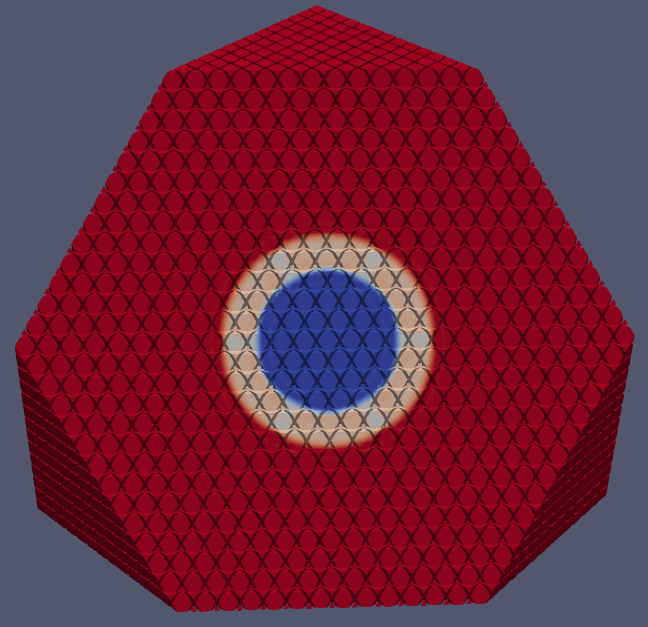
t=0.0 s

t=1.0 s

The computed energy of the 3D Euler equation at times t=0.0 s and t=1.0 s.