|
Peano
|
|
Peano
|
Very simple benchmark with a time-invariant solution subject to a shift that we can use to assess the convergence order.
The ExaGRyPE Gauge wave test is a relatively simple setup, where we employ a regular mesh over the unit square. The computational domain is centered around the origin of the coordinate system. It is supplemented with periodic boundary conditions all all sides. In theory, the wave we simulate should be a standing wave leaving the domain on the right and re-entering it on the left. If the wave shape or its amplitude change over time, this is due to numerical effects. The setup is thus convenient to assess properties of different numerical schemes.
Peano has to be built with the ExaHyPE extension plus the tracers, i.e. with
It is reasonable to start the Python script with the –help option once to see what variants are on the table. For most of my experiments, I stick to all the default settings, but I manually enable the tracers, as these allow me to track the simulation behaviour in time elegantly (see postprocessing discussion below):
The initial export is important, as we use the bespoke CCZ4 solvers from the whole CCZ4 application (even though we only use a few hard-coded experiments).
The following statements remove all the glue code and autogenerated C++ files. There is no risk in deleting them - if you rerun the Python script, they will all be reinstantiated.
To get rid of the output files, type in
The code writes the sample results into a csv file upon completion. You can use Peano's pre-manufactured postprocessing scripts to get a first impression of the solution's behaviour. The call to the script is similar to
with appropriate pathes and filenames set.
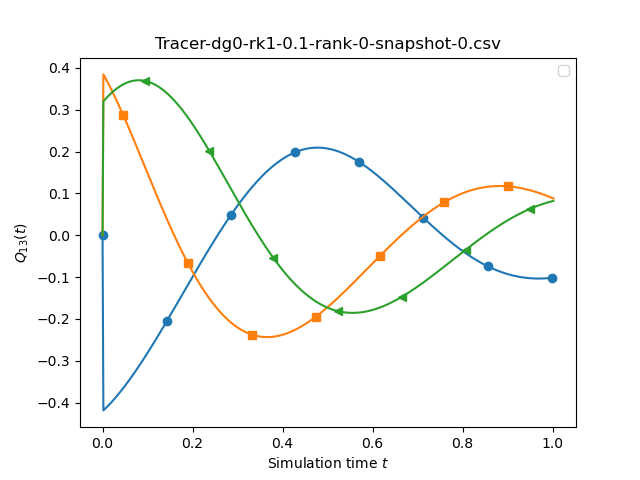
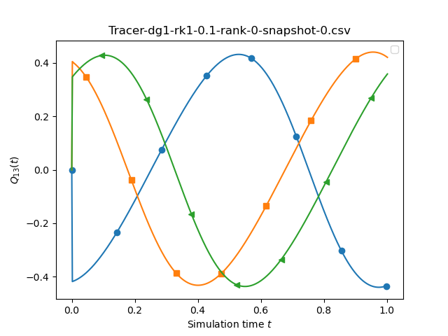
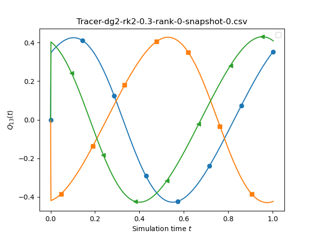
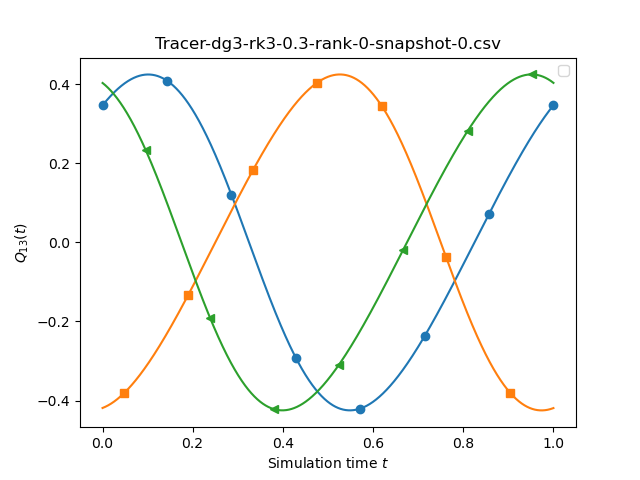
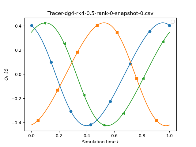
You should obtain pdfs and pngs that resemble the following graphs:
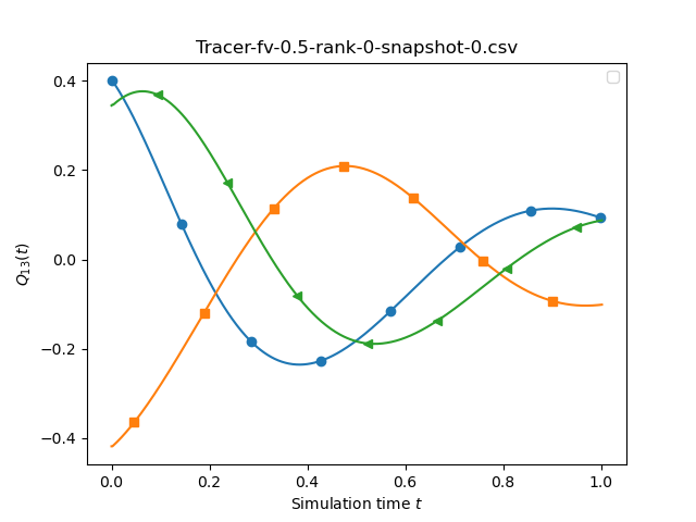

The above graphs compare the outcomes of a finite volume code (left) to the outcomes of a DG0-RK1 code (rigth). The mesh is chosen as 0.5 (FV) vs 0.1 (DG) with the default patch size of 9x9x9. Consequently, the two simulations work on exactly the same spatial discretisation. As DG0-RK1 degenerates to a plain Finite Volume scheme, the graphs should be exactly the same, and we observe that this is indeed the case.
Though the graphs simulate only a very brief total time (up to end time 1.0), we already see a strong damping of the amplitudes. This is a characteristic property of first-order (Finite Volume) schemes.
In the Python script, we played around with piecewise constant interpolation onto the tracer vs. piecewise linear. Despite the relatively coarse resolution, the graphs were all basically identical, i.e. the default resolution is already sufficient to study the long-term behaviour of the solution.

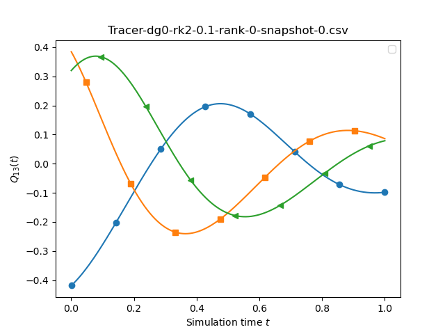
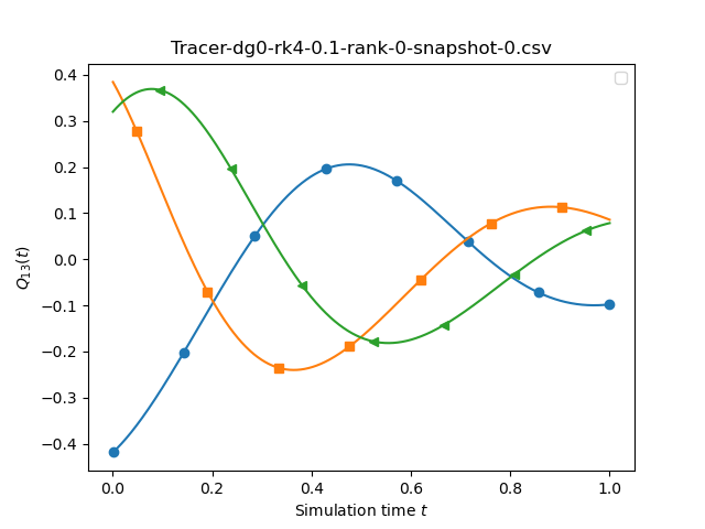
The script also allows you to compare different temporal orders. All the plots above are for different time integration orders (1,2,4) and it is close to impossiblet to spot a difference between those sketches. We we may conclude that the temporal discretisation error is not the (solve) dominating issue here.
If we compare runs with different spatial orders we see a stronger variation. This time, we compare dg0-rk1, dg1-rk1, dg2-rk1 and dg3-rk1 and set the underlying mesh size to 0.1, 0.1, 0.3, 0.3, 0.5.


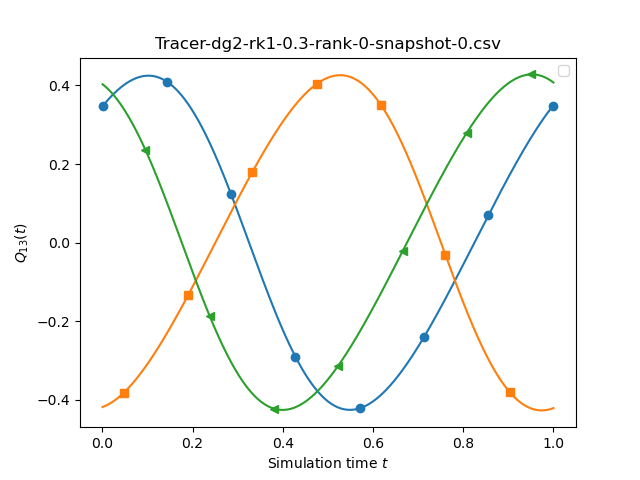

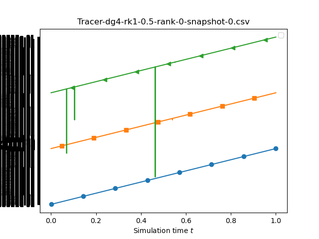
Obviously, these comparisons are not fair, and would require a more involved convergence study.
We finally increase the time stepping accuracy with the spatial accuracy, i.e. study DG1-RK1, DG2-RK2, DG3-RK3 and DG4-RK4. Again, we stick to the mesh sizes from above.
